 ©
©
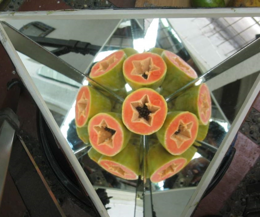
Kaleidoscopical reflections in 3 mirrors
with dihedral angles of 72° each.
| Site Map | Polytopes | Dynkin Diagrams | Vertex Figures, etc. | Incidence Matrices | Index |
©
Kaleidoscopical reflections in 3 mirrors
with dihedral angles of 72° each.
Wythoff's construction of polytopes is closely related to their reflection generated symmetry. Reflection generated symmetry groups have been listed by Coxeter and are conveniently represented by their Dynkin diagrams. The Dynkin diagram is kind of a dual representation of the mirror setup.
The general Dynkin diagram of a locally 2-dimensional symmetry for instance is given by
    o
   / \
  p   q
 /     \
o---r---o
where each node o symbolizes a mirror of symmetry and the numerical markings at the link between any two nodes give the fraction of a half circle about which the corresponding mirrors are slanted to each other. In order to get a closed trip around such a mirror crossing, the number has to be a rational larger than 1 (as 1 would mean 2 coplanar mirrors which thus could be identified and have not to be given twice). For more notational ease, links which would have been marked by 2 (perpendicular mirrors or a dihedral angle of 180°/2 = 90°) are commonly not drawn at all, and at links marked by 3 (dihedral angle of 180°/3 = 60°) the number is often omitted.
The Dynkin diagram here is a representation of the fundamental domain of the symmetry group. This is true for any dimension, where nodes still represent mirrors, and drawn links represent non-right angles between those mirror (hyper)planes.
The higher the dimension the more loops and bifurcation points might remain in the diagram, even if links marked 2 are omitted. Such a diagram is not well suited for inline notation. The easiest way to get down to an inline representation which moreover works throughout all possible Dynkin diagrams is to virtually strip the diagram into several threads. This can be done by selecting offending multi-furcating links or loop-closures and separate them virtually from one of their nodes. To that open ended link a new virtual node is attached which identifies to which real node it has to be re-attached. Those identifiers are given by asterisks followed by the alphabetical position number of the referred real node, counted from the left throughout the whole inline symbol. If a diagram has dimensional equivalents it might be useful to have negative position numbers for counts from the right hand side too. Node referees are given in lower case letters, parameters for link marks in upper case letters.
The above diagram would thus be denoted linearized by
oPoQoR*a  =  *-aPoQoRo  (linearized symbols)
a b c            c b a  (referred positions)
The set of irreducible discrete reflection-generated pointgroups of arbitrary dimension are known to be the following Coxeter groups. The left group names are according to Coxeter himself; in parantheses the slightly differing Lie group names are added.
A(n)  (= An)    or  o3o...o3o                                                        (n>0 nodes)
B(n)  (= Dn)    or  o3o...o3o *b3o      =  o3o...o3o *-c3o      =  o3o3o *b3o...o3o  (n>3 nodes)
C(n)  (= Bn)    or  o3o...o3o4o         =  o4o3o...o3o                               (n>1 nodes)
D(2)p (= I2(p)) or  oPo
E(6)  (= E6)    or  o3o3o3o3o *c3o      =  o3o3o3o3o *-d3o      =  o3o3o3o *b3o3o
E(7)  (= E7)    or  o3o3o3o3o3o *c3o    =  o3o3o3o3o3o *-d3o    =  o3o3o3o *b3o3o3o
E(8)  (= E8)    or  o3o3o3o3o3o3o *c3o  =  o3o3o3o3o3o3o *-d3o  =  o3o3o3o *b3o3o3o3o
F(4)  (= F4)    or  o3o4o3o
G(3)  (= H3)    or  o3o5o
G(4)  (= H4)    or  o3o3o5o
These are all of finite order. In fact, the respective orders can be given by the following listing:
|I2(p)| = 2p                         e.g. |I2(3)| = 6; |I2(4)| = 8; |I2(5)| = 10; ...
|An|    = (n+1)!                          |A1| = 2; |A2 = I2(3)| = 6; |A3| = 24; |A4| = 120; ...
|Bn|    = 2n n!                            |B2 = I2(4)| = 8; |B3| = 48; |B4| = 384; |B5| = 3840; ...
|Dn|    = 2n-1 n!                          |D3 = A3| = 24; |D4| = 192; |D5| = 1920; ...
|En|    = ∏ [1,2,6,10,16,27,56,240]n      |E4 = A4| = 120; |E5 = D5| = 1920; |E6| = 51,840; |E7| = 2,903,040; |E8| = 696,729,600
|F4|    = 1152
|Hn|    = ∏ [2,5,12,120]n                 |H1 = A1| = 2; |H2 = I2(5)| = 10; |H3| = 120; |H4| = 14,400
where ∏ [...]n represents the product of the first n list entries.
In addition there are the infinite ones with translational symmetry, where the corresponding (affine) Weyl group symbol is given in addition at the right.
P(n)  or  o3o...o3*a                                        or  An-1  (n>2 nodes)
Q(n)  or  o3o...o3o *b3o *-c3o  =  o3o3o o3o3o *b3o...o3*e  or  Dn-1  (n>4 nodes)
R(n)  or  o4o3o...o3o4o                                     or  Cn-1  (n>2 nodes)
S(n)  or  o3o...o3o4o *b3o      =  o3o3o *b3o...o3o4o       or  Bn-1  (n>3 nodes)
T(7)  or  o3o3o3o3o *c3o3o                                  or  E6
T(8)  or  o3o3o3o3o3o3o *d3o    =  o3o3o3o3o *b3o3o3o       or  E7
T(9)  or  o3o3o3o3o3o3o3o *c3o  =  o3o3o3o *b3o3o3o3o3o     or  E8
U(5)  or  o3o3o4o3o                                         or  F4
V(3)  or  o3o6o                                             or  G2
W(2)  or  o∞o                                               or  A1
The dotted ellipses in the above representations always are to be filled with some number of connectors all with markings "3". For instance the diagrams of B(6), E(6), resp. P(4) usually would read without that linearization
              3-o                o              o--3--o
             /                   |              |     |
o-3-o-3-o-3-o     B(6),          3      E(6),   3     3   P(4)
             \                   |              |     |
              3-o        o-3-o-3-o-3-o-3-o      o--3--o
Coxeter groups act in n-dimensional Euclidean spaces, n according to the number given in the parentheses, because pointgroups clearly are restrictable to the surface of the corresponding unit hypersphere. The origin, outside that sphere, remains fixed (thereby providing the name point group). The Weyl groups also act within n-dimensional Euclidean spaces, where n still is according to the number given in the parentheses. Here the notation with paranthesis is due to Witt, while that with subscript belongs to Weyl. For those infinite groups there is no fixed element any more. Their translational part thus can be seen like using that Euclidean space as a hypersphere of one dimension plus, but having an infinite radius and thus just becoming flat. This is why Dynkin symbols of Weyl groups always use one node more than the dimension of acting space.
Coxeter groups generally are related to polytopes by means of the kaleidoscopic construction of Wythoff. Similarily then Weyl groups can provide n-dimensional flat Euclidean tesselations. But esp. in crystallography Weyl groups are also related to lattices, i.e. periodic point sets without further incidence structure. There, usually the Weyl group symbols often are transfered onto the corresponding lattice. (It should be warned though, that the usage of Bn and Cn in literature tends to be mutually inverted sometimes, both from author to author, or even within a single monograph from chapter to chapter. The above provided attribution however is in accordance to Coxeter.)
The Dynkin diagrams are a dual representation of the fundamental simplex of that pointgroup in the sense given above. Reducible symmetry groups have fundamental regions which are pyramid products of several such simplices, or, using the language of the Dynkin diagrams, those fall apart into disconnected subdiagrams (as links marked 2, which represent orthogonality, are not shown). Within the chosen linearization of diagrams this would mean that the threads fall into at least two classes where neither thread of one does refer to one of the other class.
The restriction of fundamental domains to simplices is due to the spherical or euclidean space embedding, cf. the provided reflectional symmetries above. (The only exception in Euclidean space might occur when a vertex of the simplex runs off, towards infinity.) In hyperbolic space there will be reflectional symmetries also, which have other fundamental domains, and thus cannot be described by Dynkin diagrams any longer. – Although concepts might apply beyond, we stick in the following description to simplices.
If several elementary fundamental simplices are combined to form a larger simplex – and its bounding hyperplanes will reproduce the same pointgroup – this group will give a multiple cover of the hypersphere by the larger simplices. The multiplicity clearly is given by the number of joined elementary simplices. Dihedral angles will thus be multiples of some of the elementary ones. Correspondingly the connectors in the diagrams bear markings which are submultiples of the former link marking.
Sure, it makes sense only when adjoining simplicial domains of the same symmetry group. But conversely, the resulting simplex of such an addition needs not be a generator for the full symmetry group, it might also produce a subgroup only. Although such cases are not valid fundamental domains, they are allowed to contribute for further additions (as the sum of a non-valid and a valid simplex might result in a valid one again).
For n=3 dimensional space the set of all possible fundamental regions of irreducible finite symmetry groups are known under the name of Schwarz triangles. The non-elementary ones are derived by the following additions of Schwarz triangles out of the elementary ones
    o           o            o
   / \         / \          / \
  p   q   =   p   x    +   x'  q
 /     \     /     \      /     \
o---r---o   o---r1--o    o---r2--o
where
1/r = 1/r1 + 1/r2
1 = 1/x + 1/x'
Note again, Schwarz triangles might well differ in their numbers, as representing different fundamental domains, but the generated pointgroups are only the few ones described by Coxeter (listed above). Any of those more general fundamental domains is a union of µ elementary domains (in the sense of the just given addition), µ being the multiplicity. The explicit list of Schwarz triangle addition is available too.
For n=4 dimensional space the corresponding set of all possible fundamental regions of irreducible finite symmetry groups are known under the name of Goursat tetrahedra. Goursat tetrahedra might be added according to
    o               o               o
    r               r1              r2
  p o t     =     p o t     +     x'o y'
  q   s           x   y           q   s
o   u   o       o   u   o       o   u   o
(lines omitted), where
1/r = 1/r1 + 1/r2
1 = 1/x + 1/x'
1 = 1/y + 1/y'
and
    o           o           o
   / \         / \         / \
  p   q   =   p   x   +   x'  q
 /     \     /     \     /     \
o---r---o   o---r1--o   o---r2--o

    o           o           o
   / \         / \         / \
  t   s   =   t   y   +   y'  s
 /     \     /     \     /     \
o---r---o   o---r1--o   o---r2--o
are valid equations of Schwarz triangles. (That above given equation divides the general Goursat tetrahedron (shown to the left) by a virtual plane along the edge marked r and a point on the line marked u.) The explicit list of Goursat tetrahedra addition is available too.
This is the right place to show the might of the given inline representation. No other linearization known so far is able to display a general Goursat tetrahedron. In the linearization defined above the general Goursat tetrahedron could be rewritten as
       o             a
       r             R     left:  general Goursat tetrahedron (any node is 3-valent)
     p o t         P c T   right: rewritten by assigning position characters
     q   s         Q   S
   o   u   o     b   U   d

   oPoQoSoT*aR*c *bU*d     : linearized symbol
   a b c d                 : referred positions
Wythoff constructs general uniform polytopes after the principle of kaleidoscopes. A single point (seed) is reflected by hyperplanes (mirrors), acting as generators of the point group, and produces thereby a pointset which serves as vertices of the polytope. One has to distinguish here mainly 2 different cases: either the seed is incident to a specific mirror ("on") or not ("off").
Coxeter's later representation of these states by means of marked Dynkin diagrams does represent each mirror by a node. When the chosen seed point happens to be on that mirror, the node remains unringed (inactive mirror), but when the point would be off, the node gets ringed (active mirror). The here mainly used linearization of Dynkin diagrams then represents ringed nodes instead by x and unringed ones by o.
Edges incident to the starting point are defined by the convex hull of the generating point (p) plus each of its direct mirror images (p'). All further edges then are images of this starting set. Thus the skeleton is defined.
Obviously any edge will be perpendicular to one of the mirrors. This is where the additional idea of Mrs. Krieger comes in, which does not only allow for the 2 different topological states, but even introduces some measuring. In fact, it becomes possible to refer to the size of that edge just by this very symbol x (off-ness). Thus she introduces e.g. further specific non-unit values like f (edge size being (1+sqrt(5))/2 = 1.618034), q (edge size being sqrt(2) = 1.414214), etc.
Any further of the k-dimensional elements then gets defined by recursion. Given a subset of already defined (k-1)-dimensional elements incident to the generating point which spans an affine k-dimensional hyperplane orthogonal to some of the bounding elements of the fundamental region, and which together with their (k-1)-dimensional image elements with respect to the subsymmetry of that simplex boundary surround it completely. That one then defines thereby the circumscribed k-dimensional element of the constructed polytope. Again the other ones are obtained by its reflection.
This construction gives topologically different polytopes depending on where the generating point lies with respect to the boundaries of the fundamental domains. It may lie within the inner region of the simplex itself (all nodes "off") or within the inner region of the intersection of any number of simplex boundaries (corresponding nodes "on").
The former representation by ringings of nodes of the corresponding Dynkin diagram usually meant that all edges would have been chosen equally sized. The same now becomes clearer when using the same x measure throughout (for non-o ones). That is, the seed point has to be chosen such that it is positioned at equal distance to all boundaries of the fundamental domain where it is not already coincident. For simplicial domains such a choice is always possible. It is achieved obviously by using the corresponding angle bisectors.
 |
 |
 |
© |
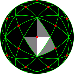
| o3x5o seed poit on mirror between π/2 and π/3 corners as well as on mirror between π/2 and π/5 |
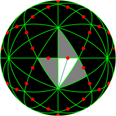
o3x5x seed point only on mirror between π/2 and π/3 |
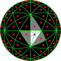
x3x5x seed poit off wrt. all mirrors |
|
|
|
|||
Simplicial domains are always necessary for spherical geometry. Even in euclidean geometry there is just a single exception to this restriction. In hyperbolic geometry so other domain types come in. But, depending on the reflection symmetry, specific edge sizes (position of seed point) might lead to degenerate singularities of topology where some elements coincide.
The requirement of equal edge lengths (just "x" or "o" only) restricts to one representant of each set of topological equivalent polytopes. Its relaxation, mentioned above, had been earlier considered already, but then not with respect to Dynkin diagrams, only with respect to the represented polytopes: This in fact is what Brückner called "Varietäten".
The construction device itself is reflecting its dimensional hierarchicality. Restricting oneself to the subspace of a single mirror plane, the intersections of the other mirrors will provide again a kaleidoscope within that space. So again the Wythoff construction can be done, which will result in that facet of the original polytope which is orthogonal to that mirror. So by hiding any single node of the diagram plus all links emanating therefrom, the new diagram correlates to that very facet. Even the vertex figure can be derived from the Dynkin diagram.
For the context of incidence matrices one has to be careful with numbers being 2 (the links of which usually are completely omitted), as triangles etc. are full valid faces, whereas a digon (x-2-o) degenerates to a doubled edge, and thus might be replaced by an element of smaller dimension. On the other hand an alternate bi-digon (x-2-x), i.e. a rectangle, is still full dimensional. So coming back to the reduced Dynkin diagrams where links marked 2 are omitted, we have the rule that any disconnected subdiagram has to have at least one node ringed.
|
External links |

|
Due to the fact that the hypercubical symmetry just represents the way the euclidean (i.e. orthogonal) coordinates are set up, it becomes evident, that there has to be a quite easy way to derive the polytopal coordinates from the Dynkin symbol directly. In fact, take the symbol to start with the -4- link. Then the coordinates of the first vertex of the (unit edged) polytope could be derived such:
(All other vertices are derived therefrom by all sign changes and all coordinate permutations.)
As an abstract polytope a digon clearly is a valid entity. Moreover, any 2 abstract poytopes would be different entities, when one contains at least a digon, while the other is obtained from the former abstract polytope by reduction of that face and unification of its bounding edges: the element counts clearly differ.
With respect to geometric representation spaces the thing becomes a bit different. For any 2 points in general position (that is, not being coincident, nor being opposite points – if the latter would be possible), there is exactly a single line running through both. Therefore a digon with those points as vertices will always have zero area, respectively their bounding edges will be coincident. So in geometric representation spaces these 2 abstract polytopes, mentioned in the paragraph before, will look exactly the same. Or, the other way round, if one uses abstract polytopes only for descriptions of real ones, so far there will be no need for digons at all.
This ease also makes Dynkin symbols much easier to denote. Else one would need for an n noded diagram n(n-1)/2 links. But usually most of those bear a link label 2, and this ease allows to omit these links in the diagram. Regular polytopes thus can be denoted by linear diagrams (with one end-node being ringed only), the precondition for the setup of Schläfli symbols.
None the less there is a singular case in geometric representation spaces, there digons come in with non-empty area. In fact this is a continuous infinitude of digons. For in spherical geometry there can be opposite points (pols). Those can be joined by different edges (meridians), in fact emanating from either point at any angle.
Whenever there is some operation of a modulo wrap considered for spherical space (sub-)elements, like alternations or especially identifications of opposite points in elliptical space polytopes, then digons always play a role not to be neglected.
The earliest systematical interest on polytopes even of higher dimensions was restricted to regular ones mostly. Thus one was interested only in reflectional groups which show up a linear form for free, and moreover the single marked node within the Dynkin description is one of the 2 end nodes. Surely the symbol might be oriented with the marked node to the left. In such a setup neither the ring nor the nodes at all are any longer needed. Although being historically right the other way round, here the Schläfli symbols might be derived as special cases of Dynkin diagrams. We have
{P,Q,...,R,S} = xPoQo...oRoSo
Gosset extended Schläfli's notation to rectified polytopes. This was done by folding the Dynkin diagram over, so that the still single ringed node would become the left-most one. He even extended this process still further to any Dynkin diagram with just a single node marked. Some characteristic examples are given below.
|
{
|
P,Q,...,R |
}
|
= oRo...oQoPxSoTo...oUoVo |
| S,T,...,U,V |
|
{
|
P,Q,...,R | S,...,T |
}
|
= oRo...oQoPx *aSo...oTo *aUo...oVoWo |
| U,...,V,W |
Obviously these later Schläfli symbols themselves neither lend to inline notation nor do they extend to more general polytopes. For instance any Dynkin diagram with more than one node ringed or any snub symbol is not describable in this way. At least if one would not use Coxeter's brute truncational notation (which btw. can be seen as a transitional stage towards the Dynkin diagram)
t0,1,3{P,Q,R,S} = xPxQoRxSo
|
External links |
|
Commonly ascribed to Wythoff himself but in fact also due to Coxeter, together with Miller and Longuet-Higgins, is the notation which attempts to describe decorated Schwarz triangles. So they could represent the mirrors of the group by the submultiple of the opposite angle of the Schwarz triangle (this is what would not work in higher dimensions). What the Dynkin diagram denotes as unringed respectively ringed nodes (or in the inline representation given by "o" versus "x"), i.e. a generating point of the kaleidoscopical construction being off respectively on that mirror, will be given in arbitrary order before respectively behind a vertical bar. So, in the dodecahedral symmetry group he would write
3 | 2 5   =   o3o5x   (doe)
2 3 | 5   =   o3x5x   (tid)
3 5 | 2   =   x3o5x   (srid)
2 3 5 |   =   x3x5x   (grid)
| 2 3 5   =   s3s5s   (snid)
Note that this notation does not lend itself for higher dimensional polytopes as well. It is restricted to the 3-dimensional case only.
|
External links |
|
There are several different snubbing procedures in common use. The one known best is the ancient one and produces the snub cube (snic) or the snub dodecahedron (snid) by kind of an alternation process. Those can be denoted as
snub( x3x4x ) = s3s4s respectively snub( x3x5x ) = s3s5s
and is produced from the omnitruncate x3x4x (girco) respectively x3x5x (grid) by a partial truncation which cuts off every second vertex down to the neighbouring vertices. Thus the x3x, x4x respectively x5x faces of the omnitruncates reduce to triangles, squares or pentagons, and in addition the vertex figures of the omitted vertices occur as well. The square faces x . x of the omnitruncate thereby degenerate to a coincident edge pair which usually is identified. Therefore the added snub triangles do meet in pairs at this places. Note that this derivation so far is still not complete, for the so derived edge lengths do clearly vary. But at least in 3D it is possible to resize those lengths without destroying the overall combinatorical structure. It is the thus varied figure what finally is called the snub.
Right in the same way the antiprisms (n-ap) or the icosahedron (ike) are derived as snub( x xNx ) = s2sNs respectively snub( x3x3x ) = s3s3s.
For the omnitruncated Wythoffians the relative coordinates of the seed point wrt. the fundamental domain was clearly its incenter (same distance to all its boundary mirrors). Because snubs however do not use every fundamental domain any longer, rather only re-use every alternate, the relative position of the seed point for an uniform snub (all edges of the same length) differs from the former. Within 3D, where those requirements do not exceed the degrees of freedom, those still can be given in a general way. Let ξi denote the distance of that point from the respective corner of the fundamental spherical triangle oPoQo; then one has
xPxQx :   sin(ξ1)sin(π/2P) = sin(ξ2)sin(π/2Q) = sin(ξ3)sin(π/4)
sPsQs :   sin(ξ1)sin(π/P)  = sin(ξ2)sin(π/Q)  = sin(ξ3)sin(π/2)
Aside it should be noted that for orthogonal products snubbing is not a commutative operation, i.e. the product of snubs is not equal to the snub of a product. Therefore they have to be distinguished in their notation. This is why the seemingly redundant link mark "2" was given in snub( x xNx ) = s2sNs, implying that the product is to be snubbed. This is in contrast to sNs sMs = snub( xNx ) snub( xMx ), where separate snubs enter into the product.
On the other hand both the even prisms (2n-p) and the truncated octahedron (toe) do have different Dynkin representations. So x xNx represents the same polyhedron as x x2No, and x3x3x represents the same as x3x4o. This observation leads to a different kind of snubbing, associated to Coxeter. Here, in contrast to the former case, one does not start with an omnitruncated figure, any partial truncation is sufficient, at least iff all 2-dimensional faces are even n-gons. In terms of Dynkin diagrams this demands a link with an even number at any transition from a snub-node to an unringed node. (Because this guarantees that one can select alternating vertices around that special face.) Finally the derived snub-like figure has to be distorted to get equal edge lengths. This is possible in general iff the original polytope to be snubbed has 2 nodes marked; this was proven by Coxeter. Under these circumstances one again can pick up any second vertex of the corresponding truncate and run the same procedure as before. In this sense it is completely valid to write snub( x3x4o ) or snub( x x2No ). Sometimes one even can find the snubbing operator being more localized to the ringed nodes, so one would write something like
snub( x3x4-)-o = s3s4o or snub( x x2N-)-o = s2s2No
Note that the Coxeter snubs often can be seen as snubs in the ancient sense by using an alternate Dynkin representation of the polytope to be snubbed, just as provided for the above examples. In general Coxeter showed that for any polytope of the form x-P-x-2Q-o-M-o-N-o-... the vertex set can be indexed alternatingly. But such a figure can be uniform only, if x-M-o-N-o-... is a simplex. So far only a single Coxeter snub is known, which can get equal edge lengths but is not uniform; this is because of the vertex figure of x3x4o3o4o, which is an octahedral pyramid.
The above Coxeter snubs, i.e. having the form s-P-s-2Q-o-M-o-N-o-... nowadays sometimes also are dubbed semisnubs too. This indeed surely is better than Johnsen's attempt to redefine the more general term snubbing to mean just the combination of truncation and alternation. In fact, the historic reading nowadays then gets dubbed full snub in contrast.
Finally a further usage of a snubbing operator can be found. These are not true snubs in the older sense of being derived by screwing of faces or alternating the vertices. But in the spirit of a Coxeter derivation there are still some other figures, which show up some even n-gonal faces. Thence some other kind of demiation might be possible. Most often, and indeed by Johnson exclusively in this way, this is based on the equality of polytopes
| o3o3o *b... | = | o4o3o... |
| o3x3o *b... | = | o4o3x... |
| x3o3x *b... | = | o4x3o... |
| x3x3x *b... | = | o4x3x... |
Here the symmetry breaking group denotion to the left always is overcome with a symmetrical distribution of "x" nodes. Thus the higher symmetrical one to the right can be used as well. Only the asymmetrical decorations x3o3o *b... and x3x3o *b... would not lend themselves for such equalities. But, corresponding to the symmetry braking of the group, the polytopes would be demiations in the sense of alternations analogue to Coxeter snubs. So these demiations also could be denoted by
| x3o3o *b... | = | demi( x4o3o... ) | = | snub( x4-)-o3o... | = | s4o3o... |
| x3x3o *b... | = | demi( x4o3x... ) | = | snub( x4-)-o3x... | = | s4o3x... |
Only in this latter special case Johnson showed that it makes sense to use marked nodes and snub-parts within the same Dynkin diagram. So far this is only a mere notational matter, but this idea can be made meaningful and even be driven further.
This generalisation is known as the Klitzing snubs[1]. Thereby that idea of demiation does not need to be restricted to the alternation of vertices any longer, but could well be applied to any higher dimensional elements as well. The thus derived "snub" is easily derived from its corresponding "starting polytope", which occurs when the snubbed nodes of the Dynkin diagram of that snub all are replaced by normal ringed nodes. Next this diagram shows that the alternation takes place at those subpolytopes, which are given in the Dynkin diagram of the snub as the not snubbed part. That is, omit all "s" nodes and all related links from the diagram. The thus denoted subelement will have to be alternatingly withdrawn. (An explicit example will be given right below.) This alternated faceting now allows to cut off some kind of lacing prism, the top facet being the alternated element, and the bottom vertices all are neigbouring vertices of that element. In older days such an alternation took place with respect to vertices only, so the parts to be cut off were some pyramids only, the base of which are nothing but the vertex figures. But this restriction needs not to be required. In this new full generalisation the bottom of that lace prism is the parallel sectioning facet underneath the alternated element.
Start:        x4o3x   (sirco)
Alter:        . o3x
Get:          s4o3x = snub( x4-)-o3x   (tut)
(Note, that it can be proven readily, that those sefa (sectioning facet underneath the alternated element) will always be planar, i.e. the ends of the edges emanating from any to be alternated element will be contained within a unique hyperplane. Here it is: For unit-edged figures with Dynkin diagram containing only s and o nodes, i.e. the sefa of which is the vertex figure only, this becomes clear from the fact, that the starting figure has a unique circumradius, and all incident edges emanate 1 unit from the chosen vertex. So we have the intersection of 2 spheres, which defines the required hyperplane. The more general case, where x nodes do exist in the to be generated polytope in addition, can be reduced to this case by the Stott reduction resp. expansion of the starting figure, applied in such a way that the required element, which has to be alternated, reduces to a vertex: There the sectioning facet underneath already was proven to be planar. Then the expansion back is applied, which only moves the sub-elements of the sefa parallely out, so the final shape remains planar.)
Generally the direct application of a pure alternated faceting will not result in uniform figures any more, just as the alternation of vertices of the classical snub procedure on x3x4x (girco) will not result directly in snub( x3x4x ) = s3s4s (snic), but in a combinatorically equivalent variant (having different edge lengths). So in general too it is intended to have some variation implicitly be done afterwards, in order to come back to uniform figures.
Finally, even quarter-snubs can be thought of, if this operation takes place at more than one end of the Dynkin diagram.
But although the pure alternated faceting can be done in any case (cf. the note on holosnubs below), the possibility to apply such a desired afterwards variation depends on the degree of freedom of the derived figure. I. e. searching for uniform snubs in higher dimensions is less effective than in 3D. This is because in 3D there are 3 degrees of freedom for the generating point in the Wythoff construction for the polyhedral "Varietät" to be snubbed, opposed to at least 3 sides of its vertex figure, which have to become equal sided. In 4D there are 4 degrees of freedom for the generating point, but the vertex figure is in the best case a simplex, that is already 6 edges have to get the same length. In even larger dimensions this becomes still worse. (The same consideration applies to all the other sectioning facets to be used, for sure.)
There is still a further generalisation of the snubbing process in use, which commonly are called holosnubs. Johnson observed that restricting the snub operator to applications on those Dynkin diagrams only, which show up link-markings with even numerator at the transitions from s-nodes to non-s-nodes, is rather artificial when looked at locally. It only comes in from a global context. This is because the circuit around those polygons, which do correspond to those links, would have to be alternated, and alternation at a polygon with an odd count of vertices or edges is not possible. Nevertheless one could do the corresponding application locally only, thereby running around the polygon on and on until it closes again correctly. For odd numerators this would ask for doubling the winding number. Thereby the same elements in one circuit will be omitted, while in the other are retained. The effect of snubbing and holosnubbing at various different cases of polygons can be viewed here.
Although Johnson himself asked for this generalization way before the invention of Klitzing snubs, the same applies on those too. The main effect of this local view ends in replacing the polytope itself by some Grünbaumian double cover of it. This one thereby will have polygons with even vertex respectively edge counts only, and so the usual snub operator could be applied again. - Because of the required double covering of the starting figure, the outcome of its alternated faceting sometimes might remain such a double cover. In other cases however the alternation manages to end in a no longer Grünbaumian figure. Snubbing generally halves the vertex count, even for Klitzing snubs. Because of the double cover required for holosnub generation (running twice around in the local application) the vertex count first gets doubled and afterwards then halved. In total it comes out that holosnubbing does not change the vertex count, while snubbing does half it.
For higher dimensional examples, than just polygons, confer the parallels of the derivation of snub( x-4-)-a-3-b = s4a3b and holo( x-5-)-a-3-b = β5a3b, where "a" and "b" independently can be "x" or "o". The new node mark "β" is just used to distinguish holosnubs more significantly from the former snubbings (the relevant odd link mark in fact would be enough to do so). So for instance snubbing the small rhombicuboctahedron (sirco, for a=o and b=x) will alternate the triangles, thereby one half will be maintained as demi( . o3x ), the other half will be replaced by sefa( s4o3x ), the sectioning facets underneath and parallel to the omitted elements, which in this case are hexagons. The squares here become snub( x4o . ) = s4o ., i.e. they degenerate into edges. Thus snub( x-4-)-o-3-x = s4o3x is the truncated tetrahedron (tut) with half as many vertices (of type [3,6,(4/2,)6]) than the starting rhombicuboctahedron. This has to be paralleled to the holosnub of the small rhombicosidodecahedron (srid), where the maintained triangles demi( . o3x ) and the parallel sectioning facets underneath the omitted ones, the hexagons sefa( s5o3x ), now occur as parallel pairs in all places because of the required double circuit. The pentagons here transform into holo( x5o . ) = β5o ., i.e. become pentagrams. So the holo( x-5-)-o-3-x = β5o3x is the small icosicosidodecahedron (siid) with the same amount of vertices (of type [3,6,5/2,6]) as the starting rhombicosidodecahedron.
In order to get the alternated faceting approach more ready to hand, in the matrices the remaining elements of the alternated ones are given in bold type always. Snubs or holosnubs with the vertex count emphasized are the more classical ones. But if a higher dimensional count would be emphasized, then it was derived according to the Klitzing generalization.
For polyhedra, if applicable, pictures according to the alternated faceting approach are provided (for instance cf. "snub derivation" at the polyhedra linked above). Those pictures are color coded:
red elements          - elements to be alternated
yellow faces          - sectioning facets underneath ("sefa")
faces in other colors - remainder from the starting figure
(the starting figure still is provided as edge skeleton)
Uniform polytopes usually have high symmetry. Prisms and antiprisms show axial symmetry only. In order to extend this class of polytopes, the set of segmentotopes is designed. They are defined by three axioms only, beside of following the restrictions of being polytopes:
From that definition it follows that all 2-dimensional boundaries have to be regular polygons. That the top and bottom bases have to be either uniform polytopes or at least Johnson type hypersolids with a definit circumcenter. The lateral boundaries are segmentotopes in turn. In 2D there are only two segmentogons: the regular triangle (point atop line) and the square (line atop line).
The notion of segmentotopes was lateron expanded to orbiform polytopes: These just lack the "segment" restriction of the definition, or given the other way round, segmentotopes can nowadays be given as monostratic orbiform polytopes.
Segmentotopes are usually denoted by the pair of bases (which do not have to be unique), respective their Dynkin diagrams, like [top base] || [bottom base]. The parallel sign here is read as "atop". In the special case that top and bottom base show the same symmetry the symbol might be shortened in a way as was given by Miss Krieger for lace prisms:
o3x5o || x3o5x = ox3xo5ox&#x
here the group unifies, the top and bottom bases are given as first respectively second nodes at each position. The final &#x denotes that there are lacings joining the bases, which have the same length x as are used for the bases.
Although both concepts have a large intersection, they are not completely equivalent. For instance segmentotopes are not restricted to bases which are described by Dynkin diagrams. Diminishings, as used in the set of Johnson solids, might be applied to either base. Further, there need not be a reflection group which unifies both bases simultanuously, so that a single lace prism type Dynkin symbol could be set up. A segmentochoron, which cannot be given as such a lace prism and which is not just derived as some diminishing of the top, bottom, or of both figures, would be cube || ike. – Conversely, lace prisms are not bound to unit edges alone.
As segmentotopes by their definition are monostratic, clearly axial stacks of several segmentotopes might be considered too. If all those vertex layers show a common symmetry, the multistratic arrangement was called lace tower. Note that the layer polytopes between the uppermost and lowermost base are true facets of each lace prism, but are withdrawn in the joined stack. Sometimes one even finds the inner layers been marked as pseudo, but might be understood right from construction. Within a segmentotopal approach clearly each monostratic stack should have an individual circumradius, but in general surely not the whole tower is bound to, although those towers which do will provide especially interesting figures. As easiest example the octahedron (oct) might serve:
o4o || x4o || o4o = oxo4ooo&#xt
in the unified notation the sequence of node marks is meant for the sequence of layers. The final t reminds to interpret this symbol still axial as tower.
For lace tower descriptions, even for uniform polytopes, it is clear that the non-extremal layers are not bound to use unit edged sectioning sub-polytopes. Edge lengths which occur as chord lengths of unit-edged regular polygons are common. (And even worse, for lace towers of polytopes, which do use such different lengths for edges, e.g. lace towers of lace towers, i.e. those lace cities described below, the sectioning polytopes will use edge-lengths which occur as chords in polygons having these different edge lengths.) The most common ratios in the lower regular polygons are, using x(m,n) as the chord length of a regular m-gon when using the n-th vertex:
x(m,0) = o
x(m,1) = x
x(m,2) = x(m)
esp.     x(2)   = o
         x(3)   = x
         x(4)   = q                q : x  = 1.414214 = sqrt(2)
         x(5)   = f                f : x  = 1.618034 = (1+sqrt(5))/2
         x(5/2) = v                v : x  = 0.618034 = (sqrt(5)-1)/2
         x(6)   = h                h : x  = 1.732051 = sqrt(3)
         x(8)   = k             x(8) : x  = 1.847759 = sqrt[2+sqrt(2)]
         x(8/3)               x(8/3) : x  = 0.765367 = sqrt[2-sqrt(2)]
         x(10)                 x(10) : x  = 1.902113 = sqrt[(5+sqrt(5))/2]
         x(10/3)             x(10/3) : x  = 1.175571 = sqrt[(5-sqrt(5))/2]
         x(12)                 x(12) : x  = 1.931852 = sqrt[2+sqrt(3)]
         x(12/5)             x(12/5) : x  = 0.517638 = sqrt[2-sqrt(3)]
         x(∞)   = u                u : x  = 2
general:                        x(m) : x  = sin(2π/m) / sin(π/m) = 2 cos(π/m) for m>1
x(m,n)
esp.     x(m,m-n) = x(m,n)
         x(6,3)   = u
         x(8,3)   = w              w : x  = 2.414214 = 1+sqrt(2)
         x(8,4)   = qk        x(8,4) : x  = 2.613126 = sqrt[4+2 sqrt(2)]
         x(10,3)  = ff            ff : x  = 2.618034 = (3+sqrt(5))/2
         x(10,4)  = fx(10)   x(10,4) : x  = 3.077684 = sqrt[5+2 sqrt(5)]
         x(10,5)  = fu       x(10,5) : x  = 3.236068 = 1+sqrt(5)
         x(12,3)  = e        x(12,3) : x  = 2.732051 = 1+sqrt(3)
         x(12,4)             x(12,4) : x  = 3.346065 = sqrt[6+3 sqrt(3)]
         x(12,5)             x(12,5) : x  = 3.732051 = 2+sqrt(3)
         x(12,6)             x(12,6) : x  = 3.863703 = 2 sqrt[2+sqrt(3)]
general:                      x(m,n) : x  = sin(π n/m) / sin(π/m) for m>1 and 0≤n≤m
Beside of arranging 3 or more layers in a linear stack along a common axis, those could be arranged in a closed circular ring, in which case instead of the final t a final r is used (lace ring). They further can be used in the multiply connected form of a simplex too, that is any sub-symbol of any 2 layers is to be meant as a lace prism. Such things are called lace simplices. Denoted are those like the lace prisms by the mere suffix &#x, but like towers or rings they show up more than just two markings per node. So
oxox&#xr
has 4 layers of symbols outlined in the form of a ring, which then are laced together accordingly in a cycle. This very example however could further be reduced into 2 pairs of consecutive lace prisms (ox&#x = o3x) which as such, in correct relative placement, form the segmentohedron o3x || x3o = ox3xo&#x, i.e. the octahedron (oct). In rare examples non-simplicial higher-dimensional reconnection lacings might be required, like eg. octahedral lacing alignments. Those however so far have not been settled into a final notation and rather are to be considered individually by other means. (If needed in incidence matrices for some non-symmetrically orientated element, one might denote them simply by the suffix &#x+, simply intending for "some" higher (surplus) lacing structure.) The lace simplex
oxo&#x
denotes a tetrahedron (tet), because the point, the line and the other point all are joined together pairwise. While with an additional t this symbol would denote a planar configuration of 2 regular triangles, adjoint at one of their edges; the lacing edge between the 2 points is missing then. Lace simplices are an especially useful description in the context of vertex figures; in fact, they have been introduced right for that reason.
Lace towers or lace simplices with an pairwise offset height of zero, and further without the addition of lacing edges, i.e. the mere stack of several polytopes within a unifying symmetry, all being centered around a common center, is nothing but a compound. Accordingly, under these premises, those could be denoted accordingly, for sure lacking the suffix "&...": For instance, the stella octangula, i.e. the compound of 2 dually arranged tetrahedra, could thus be denoted as
xo3oo3ox
Sure, not all compounds can be described in this way. This description asks for an overall symmetry, under which the components themselves can be given too. As in the above example, this description serves especially well e.g. for compounds of dual pairs.
In 2014 Mrs. Krieger extended her zoo of lace prisms, towers, and simplexes a bit. She introduced a further qualifier "z" (zero). If this qualifier precedes the lacing edge lengths ("...&#zx.."), then the respective segmental heights happen to become zero. (In that this qualifier adds just some optional further information to the reader.) But there is a bit more to that: For lace prisms the bases usually are part of the figure. And for lace towers the extremal layers similarily. But not the intermediate ones. Those happen to be just pseudo facets, sectioning the tower into segments. But for degenerate lace towers there might occur situations, where this splitting of the vertex set into subsets (those co-hyperrealmic "layers") would result in pseudo facets solely. This then is a case, where this preceding "z" qualifier surely would be required! – A simple example here would be the ike, when being represented in briquet symmetry: ((fxo ofx xof))&#zx. (Where the doubled parantheses encode that none of those golden rectangles belongs to the bounding elements of ike.)
She then also allowed for a suffixing "z" too. This one would build up the structure as devised without that additional "z" first, and thereafter scales all lacing edges down, such that the segmental heights all become zero. – This probably would be rather seldomly used explicitly. But implicitly it provides a different pictoral representation for the segmentochora, in fact the "telescope view" from infinity. (The pictures provided within this website however usually provide views from nearby, thus relatively scaling the two bases additionally in a perspectivic way.)
A further concept closely related to the former zoo is that of lace cities. Here the name derives from the picturesque description of a city: being a set of towers. So re-consider the just described lace towers. If each of those layers on its own can be described as a tower, if further all those towers of one dimension less are describable within the same symmetry group, then there is an arrangement of the higher tower in the manner of a street, while the lower towers are given as sets of layers at the specific grounds. This yields a 2 dimensional graphical arrangement of Dynkin symbols, each of 2 dimensions less. Take for example the octahedron (oct). It can be given as the lace tower (in fact only a lace prism) xo3ox&#x, i.e. x3o || o3x. Now x3o = x o&#x and o3x = o x&#x. Thus we have for lace city
 x o     <- x3o
o x      <- o3x
The advantage of lace cities is that these can be freely rotated within the plane of display, and often thus provide further lace tower descriptions for free without any further considerations. In this tiny example for instance (because of x x&#x = x4o) there is likewise: o4o || x4o || o4o.
Beyond the introduction of lace towers by Miss Krieger, an extension of those even serves useful for 2-sided infinite "towers", when describing e.g. periodic honeycombs as infinite stacks of tilings. Sure, we don't want to use an infinite amount of node symbols at every node position, but here the periodicity could be used: we add a colon sign (:) for the according reduction to one period. Subelements which reside completely within that period are given as usual. Subelements, which cross the boundary of that period, will be mod-wrapped into that same period. (Be aware, that those then might even superimpose at their margins.) Here the colons will be needed to represent the mod-wrap. In addition we provide a doubling of the # symbol (&##x), representing the infinitude of the required stacking. (This usually is superfluous. But occasionally will become essentially, when thereself infinitely stacked subelements would occur.)
x4o4o  =  :x:∞:o:&##x
x4x4o  =  :wxw:∞:oqo:&##xt

x4o3o4o  =  :x:4:o:4:o:&##x
o4x3x4o  =  :qooo:4:xuxu:4:ooqo:&##xt
|
External links |
|
© 2004-2026 | top of page |
