©
| Site Map | Polytopes | Dynkin Diagrams | Vertex Figures, etc. | Incidence Matrices | Index |
In their search for abstract polytopes even the restriction to dyadicity was set apart by Shephard (1952) and Coxeter (1974). Today the outcome of their finds usually is connoted as complex polytopes. This is because e.g. an n-edge, i.e. a somehow 1-dimensional object (edge) with n 0-dimensional subelements (vertices) can easily be represented within the 1-dimensional complex "line" as the convex hull of the n roots of unity, or, in its 2-dimensional real equivalent, the Argand plane, as a convex regular n-gon. Thus indeed there is a realization of these more general abstract polytopes which is dimension respecting.
Despite the formal geniality of the complex description, there is a much more visual approach to these figures too, which moreover is quite close to Coxeter's original description of these figures. It is more in the spirit of deriving maps or skew polytopes from other polytopes. In fact the above already mentioned identification of n-dimensional complex space and the 2n-dimensional real space are being used here. Thus those complex polytopes also can be described as some selection of (in general) even dimensional elements only in a corresponding (real space) polytope (of twice the total dimension). Both, the connection to these describing (real space) polytopes and the to be applied selection of even dimensional elements here becomes of interest on its own right.
Zero-dimensional complex polytopes (or according elements of larger polytopes) clearly are zero-dimensional real elements too (as two times zero still equates to zero). Thus the realization of those vertices remain mere classical geometric points, both within complex and within real space considerations. Nothing special here. 1-dimensional elements (edges) however start to fall apart. Those have been described already in the introductory lines above. Just the special case of re-using 2-edges within the context of complex polytopes as well has to be considered separately: the according roots of unity then are just +1 and -1, i.e. are both on the real line within the Argand plane. That is, n-edges usually come out to be 2-dimensional within according real space considerations, but the special case of n=2 remains 1-dimensional within its real space embedding! For sure, such a 2-edge on its own will not be a truely complex polytope, rather it is degenerate and happens to be a real one again, but it well could be used beside others or in combination with a truely complex polytopal vertex figure. The remainder however will be devoted to higher dimensional complex polytopes of rank 2 and beyond.
The re-reading of 2{q}2 = {q} makes clear that Coxeter's notation is more based on the Schläfli symbols than on Coxeter-Dynkin diagrams. Therefore in here a mixed notation will be introduced, then re-using the typewriter friendly inline notations of the latter being applied to the former: Note that Schläfli symbols are meant to describe regular polytopes only and that their (single) "ringed node" (then denoted by x) always is situated at the left-most position and that conversely all other nodes therefore get "non-ringed" (i.e. represented by o). Thus we become able to rewrite the general complex polygon from now on as p{q}r ≡ xp-q-or instead. And similarily for higher dimensional complex polytopes.
Such a rewrite then allows us to consider non-regular complex polytopes as well, such as truncations thereof, etc. What does mean to "truncate" a complex polytope? In fact it is analogue to the real space case: The former edges become somewhat smaller (or alternately get pulled somewhat out so that their former vertex incidences get lost), those former vertices then get replaced by their vertex figures, and the facet polytopes get truncated in turn, thereby defining a dimensional recursion down to the 2-dimensional case, which then becomes trvial, as here the facets are just those already mentioned edges. Note, that the terms edges, vertex figures and facets do apply within a complex polytopal setting right the same. Just that we consider more general n-edges rather than 2-edges only. Moreover, it becomes clear that the same considerations would apply for any other Wythoffian decoration, i.e. any other Stott expansion / contraction as well.
It is only when it comes to such Wythoffian decorations, that multiple ringed nodes of the according Coxeter-Dynkin diagrams not only come into consideration, but also into mutual interaction. And only then there rises the question about their respective sizes, esp. if nodes with different indices get involved. A premature decision might argue, that if the real edges had a circumradius size = 1/2 (of edge length units), one might use for other n-edges the same circumradius scaling too. However, as we want here to show up as often as possible the relation between a complex polytope and its real space embedding, and it is that those are usually known better for their unit-edged variants, it is that we rather choose in here that relative scaling of n-edges, which asigns to them the radius of the according real space n-gons instead. I.e. the circumradius of an n-edge gets the metrical property of 1/(2 sin(π/n)).
Within Coxeter's description these are denoted p{q}r and represent an abstract "q-gon" (the understanding of that number still has to be given) which uses p-edges, i.e. "edges" with p incident vertices each, and having r such edges incident to every vertex. So, within the usual realm of real polygons, where dyadicity always holds, we clearly have p=r=2 and therefore 2{q}2 is nothing else than the usual polygon {q}.
These numbers p,q,r of Coxeter's notation in fact originate from their group description. In fact, if its 2 generators are A,B, then they just tell Ap = Br = id. Further, if q is even, then additionally holds (AB)q/2 = (BA)q/2, while if q is odd, then instead (AB)(q-1)/2A = (BA)(q-1)/2B.
Coxeter further provides the additional restriction pq+2pr+qr > pqr (or equivalently 1/p + 2/q + 1/r > 1) for finite complex polygons.
In fact, it only was J.G. Sunday in 1975, who gave a clear geometrical understanding of that number q, in that it can be described as the girth of the complex polygon xp-q-or, i.e. the number of vertices within a minimal cycle such that every two, but not three, consecutive vertices belong to a p-edge.
It shall be mentioned that whenever q is odd, within xp-q-or one obtains for the underlying groups, and thus for those (non-starry) complex polygons too, the further requirement that p=r, or, told differently, only for even values of q those numbers p,r could be different at all. Furthermore, under the restriction p=r any complex polygon generally does get an additional color-symmetry, which allows to alternate its (complex) edges. Thus one becomes able to consider s-nodes (snub operation) for complex polytopes as well.
Further one has to be careful about q=2 in here. For real space polygons, one generally is used to consider x2 x2 (cartesian or prism product of 2 edges) and x2-2-y2 (the rectangle with some according scaling of respective edge sides) to be exactly the same, simply because the former describes 2 independent factors whereas the latter already describes a single entity of a fixed mutual scaling. In the context of complex polygons however xp xr still generally is valid, in fact it simply can be embedded into the real space polychoron (p,r)-dip as the subset of its vertices plus its p- and r-gonal base faces, the latter of which then representing the p- and r-edges respectively. Thence its incidence matrix clearly is
pr | 1 1
---+----
 p | r *
 r | * p
The complex coordinates then simply are
(εpn/(2 sin(π/p)), εrm/(2 sin(π/r))) for any 1≤n≤p and any 1≤m≤r, where
εp=exp(2πi/p)
and εr=exp(2πi/r) respectively.
Accordingly its circumradius is sqrt[1/(4 sin2(π/p))+1/(4 sin2(π/r))].
But, wrt. an additional 2-fold symmetry element, which shall exchange these edges via a further isomorphism, it becomes clear, that it only could exist whenever p=r. Therefore, this complex polygon in general would not be regular, rather it is just an isogonal one. That is after all, for regular complex polygons the above restriction (then obtained for odd q) also applies for q=2 as well. Within that restriction however one generally has xp xp = xp-2-yp for any p, which, under the in here chosen assumption of same edge sizes (x=y), then could further be extended by xp-4-o2 = xp-2-xp.
Finally there is an equation, which relates those numbers p,q,r to the group order g and to the so called Coxeter number h.
h = 2 / [1/p + 2/q + 1/r - 1]
g = 2h2/q
That h just happens to be the number of (real) edges of the Petrie polygon of the real space representation of that complex polygon. I.e. any complex polygon might be represented as a 2D projection of its real space embedding with an h-gonal symmetry.
Assuming p,q,r,h,g all to be integers (both finite as well as greater or equal 2) we have just a few classes of solutions. By symmetry let's assume p≥r for the following classification, i.e. transfering their distinction simply to the to be applied node decorations. Then
None the less, it still is a good idea, to enlist all those here individually in tabular form additionally, because such a table shows more clearly the respective Wythoffian relationships within each of those famillies.
| non-starry | |||||
|---|---|---|---|---|---|
| o3-3-o3 | o3-4-o3 | o3-5-o3 | o3-6-o2 | o3-8-o2 | o3-10-o2 |
type B x3-3-o3 (Möbius-Kantor polygon) x3-3-x3 †) |
type E x3-4-o3 x3-4-x3 s3-4-o3 |
type B x3-5-o3 x3-5-x3 †) |
type F x3-6-o2 o3-6-x2 x3-6-x2 *) o3-6-s2 |
type F x3-8-o2 o3-8-x2 x3-8-x2 *) o3-8-s2 |
type F x3-10-o2 o3-10-x2 x3-10-x2 *) o3-10-s2 |
| o4-3-o4 | o4-4-o3 | o4-6-o2 | o5-3-o5 | o5-4-o3 | o5-6-o2 |
type B x4-3-o4 x4-3-x4 †) |
type E x4-4-o3 o4-4-x3 x4-4-x3 *) s4-4-o3 o4-4-s3 |
type F x4-6-o2 o4-6-x2 x4-6-x2 *) o4-6-s2 |
type B x5-3-o5 x5-3-x5 †) |
type E x5-4-o3 o5-4-x3 x5-4-x3 *) s5-4-o3 o5-4-s3 |
type F x5-6-o2 o5-6-x2 x5-6-x2 *) o5-6-s2 |
| op-4-o2 | op-2-op | op or | o2-q-o2 | lace prisms ‡) | |
type D xp-4-o2 (γp2, Shephard's generalised square) op-4-x2 (βp2) xp-4-x2 *) sp-4-o2 op-4-s2 |
type C xp-2-xp |
xp xr *) xp xp |
type A x2-q-o2 x2-q-x2 s2-q-o2 **) s2-q-s2 |
xp || op xp || xp | |
For sure, the individual details of those are to be provided much more explicitely. Still, because being polygons only, these are not too "structured" (in the sense of an incidence matrix) and thence do not require individual files. Rather they will simply be given below directly (as was done too for the real space polygons as well, i.e. the type A from above).
*) The ones marked such are not regular complex polygons, they rather are just isogonal ones only.
In fact, the outer symmetry between their edges xp and xr would be missing.
**) It's a classic fact that for these real space snubs only even values of q can be used for non-starry results,
as alternation only then closes back within the right parity.
†) Snubs of the form sp-q-op seem not to exist for odd
values of q in general.
At least for p=q=3 this is clearly evident, as the vertex count of its pre-image is 8 and a snubbing node
sp would require that to be multiplied by 1/p; but 8/3 clearly is not integral.
‡) For lace prisms the lacing edges, which generally still remain real ones only, cannot be mapped
by any outer isomorphism onto the p-edge(s), if p > 2. Thence those will never be regular.
In the case of non-equal bases they even would fail to be isogonal.
The first given polytope (i.e. type D above) can be understood as the selection of the p-gons from the p-gonal duoprism. In fact, these (real space) p-gons represent the (complex polytopal) p-edges, i.e. "edges" with p incident vertices, and moreover there are indeed exactly 2 such p-edges incident to every vertex.
Obviously its incidence matrix thus is
p2 |  2
---+---
p  | 2p
Note that this realization supresses the toroidal skin of the p-gonal duoprism, i.e. all its squares.
So we have (real) 4-gonal pseudo faces all over.
Or, stating it the other way round, these complex polygons simply re-use the even-dimensional elements of all the p-gons of those real duoprisms.
–
Those polytopes are the (complex) 2-dimensional versions of Shephard's generalised hypercubes
(cf.

![]() ).
In fact, p=2 not only returns into the real subspace only, but moreover becomes nothing but the well-known square.
).
In fact, p=2 not only returns into the real subspace only, but moreover becomes nothing but the well-known square.
h = 2p
g = 2p2
The above given identities directly derive from the already mentioned fact that xp xr is real space embeddable into the (p,r)-duoprism, here for p=r, and as such already was mentioned there too. In fact this latter equality of edge types then provides rise for the then possible denotation with q=2 as well. Thus providing the respective incidence matrix here as
p2 | 1 1
---+----
p  | p *
p  | * p
The complex coordinates then simply are
(εpn, εpm)/(2 sin(π/p)) for any 1≤n,m≤p,
where εp=exp(2πi/p).
Accordingly its circumradius is 1/[sqrt(2) sin(π/p)].
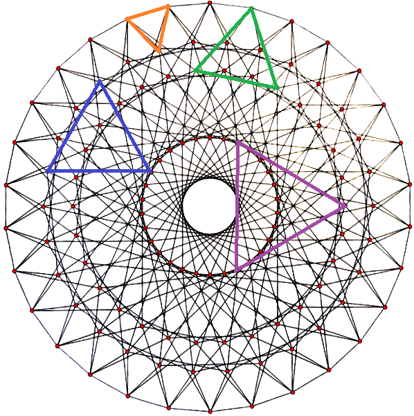
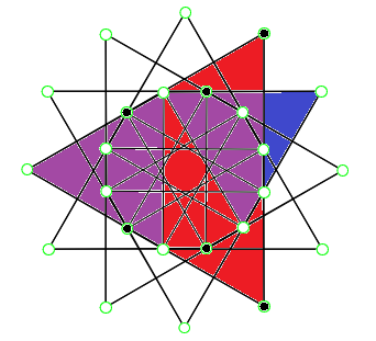
This polytope, aka the Möbius-Kantor polygon
(cf.
![]() ),
belongs to the above type B.
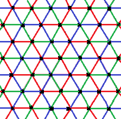
It can be understood as the selection of 8 out of the 32 triangles of hex.
Within the projection of hex, given at the right, these mentioned 8 triangles
are being represented as those 8 which are projected undeformed (up to mere total scalings), i.e. the small ones with red and the large ones with blue outlines.
In fact, these triangles represent the 3-edges, i.e. with 3 incident vertices, and moreover there are indeed exactly
3 such 3-edges incident to every vertex. –
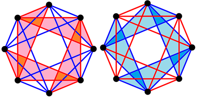
The second picture pair shows the same 3-edges projected in such a way that they become all alike, however asymmetrical triangles instead.
),
belongs to the above type B.
It can be understood as the selection of 8 out of the 32 triangles of hex.
Within the projection of hex, given at the right, these mentioned 8 triangles
are being represented as those 8 which are projected undeformed (up to mere total scalings), i.e. the small ones with red and the large ones with blue outlines.
In fact, these triangles represent the 3-edges, i.e. with 3 incident vertices, and moreover there are indeed exactly
3 such 3-edges incident to every vertex. –
The second picture pair shows the same 3-edges projected in such a way that they become all alike, however asymmetrical triangles instead.
Obviously its incidence matrix thus is
8 | 3
--+--
3 | 8
Note that those 8 to be selected triangles of hex will just form a subset of its 32 triangles. However the sides of those selected ones do form a division without remainder of the set of its 24 edges: every single edge will be incident to exactly one such selected triangle (despite the fact that in hex every edge clearly is incident to 4 triangles). Confer also the accordingly subsymmetric incidence matrix of hex together with the here required selections.
h = 6
g = 24
Further one obtains from that real space embedding directly its circumradius too, thus being just 1/sqrt(2) = 0.707107.
This polytope, again belonging to type B above, can be understood as the selection of 24 out of the 72 squares of gico, i.e. the compound of 3 teses within an ico. Note that both use the same (real) edge skeleton. In fact, the squares of the former are nothing but the diametrals of the oct cells of the latter. Within the projection of ico, given at the right, these mentioned 24 squares are being represented as those 24 which are projected undeformed (up to mere total scalings), i.e. the smaller ones with red and with green outlines, as well as the bigger (centrally overlapping) ones with yellow and with blue outlines. In fact, this subset of squares represents the 4-edges, i.e. which have 4 incident vertices, and moreover there are indeed exactly 4 such 4-edges incident to every of their vertices.
Obviously its incidence matrix thus is
24 |  4
---+---
 4 | 24
In order to understand the lifting of this selection we present at the right both the projection of any of the inscribed teses (1st pic) and the (real) 4-dimensional realization of the complex 2-dimensional polygon x4-4-o2, i.e. the 4-gonal duoprism or tes (2nd pic). As any vertex of ico belongs to exactly 2 teses of gico we thus have 4 colored (real) squares (i.e. complex 4-edges) per vertex.
Note furthermore that the holes in this encasing ico are all its (real) 3-gonal pseudo faces.
The complex coordinates, easily derived from gico (or its hull: ico)
then simply are
(ε8n, 0) for any 1≤n≤8 even,
(0, ε8n) for any 1≤n≤8 even, and
(ε8n, ε8m)/sqrt(2) for any 1≤n,m≤8 odd,
where ε8=exp(2πi/8)=(1+i)/sqrt(2).
Both, from these coordinates as well as from its given real space embedding, one obtains its circumradius to be just 1.
h = 12
g = 96
This polytope, belonging to type E above, can be understood as the selection of 24 out of the 96 triangles of ico. Within the projection of ico, given at the right, these mentioned 24 triangles are being represented as those 24 which are projected undeformed (up to mere total scalings), i.e. the ones with red, with green, and with blue outlines. The latter ones even are shown filled. (Note that this coloring is applied only for the ease of recognition here and will have nothing to do with the 4-coloring mentioned below!) It should be emphasized here, that the thus to be selected faces only provide 3 times 24, i.e. just 72 out of the 96 (real) edges. Only those have been shown in this projection pic. – These 24 triangles then represent the 3-edges, i.e. with 3 incident vertices, and moreover there are indeed exactly 3 such 3-edges incident to every vertex.
Obviously its incidence matrix thus is
24 |  3
---+---
 3 | 24
The lifting of this selection can be understood by a 4-coloring of ico. We start with the 4-coloring of oct: simply color opposite faces alike. This scheme can be extended to all cells of ico consistently using the obvious color matching rule of rotated copies only. In fact, diametrically opposite octs at a vertex figure then will be nothing but a shifted copy with an axially skrew quarter turn. – The required subset then is the selection of just one of those colors from these subsets of triangles.
Further we note that 3 such octs and thus 3 differently colored triangles will be incident at each edge of ico. Therefore each edge could be colored as well easily by applying the missing 4th color. And when turning to the vertex figure, which is a cube, then it becomes evident that the edges of such a cube correspond to the vertex-incident triangles of the ico. So those 12 edges each are colored accordingly, 3 from each color. In this coloring of the cube the 3 of either single color then happen to be the alternating ones of its Petrie polygon. (The remaining ones of that very Petrie polygon are all the other colors, one each.)
The comparision of the here being displayed projection pictures each, of x4-3-o4 (all edges) and that of x3-4-o3, exhibits that in the latter case exactly 1 (real) edge of each selected square of the former has been omitted. Moreover it appears that those omitted edges form 4 complete hexagons, which have no vertex in common, and thus in total visit each vertex exactly once. And indeed such hexagons occur as flat equatorial pseudo faces within each co, which in turn is the flat equatorial pseudo facet of ico. In fact there are 16 hexagonal great circles in the edge set of ico. These fall into 4 sets of 4 with disjoint vertices. These simply correspond to the 4-coloring of the edges mentioned in the former paragraph.
(The complex coordinates here clearly are the same as for x4-3-o4. Moreover its circumradius then will be 1 as well.)
h = 12
g = 72
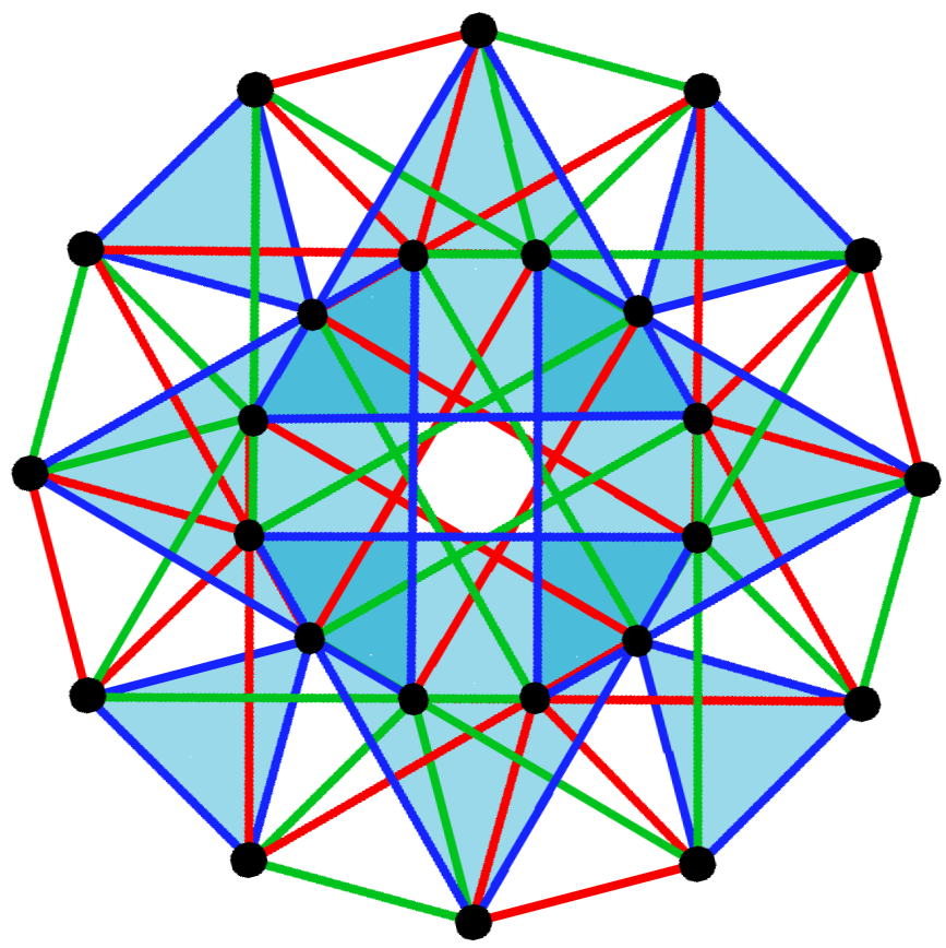
This complex polygon belongs to the type B above. It is to be obtained as substructure of gohi. Cf. the right projection thereof. Denote the subset of vertices from outside to the center as A, B, C, D. Then spot out the 30 pentagons each of types AABCB (orange), AACDC (green), ABDDB (blue), and BCDDC (purple), those are the to be chosen ones, connecting (as a complete set) mutually by 5. In fact its incidence matrix happens to be
120 |   5
----+----
  5 | 120
h = 30
g = 600
From its real space embedding one readily derives its circumradius to be (1+sqrt(5))/2 = 1.618034.
This complex polygon is the last of the ones of type B above. It is to be obtained as substructure of ex. Cf. the right projection thereof. Denote the subset of vertices from outside to the center as A, B, C, D. Then spot out the 30 triangles each of types AAB (orange), ACC (green), BBD (blue), and CDD (purple), those are the to be chosen ones, connecting (as a complete set) mutually by 3. In fact its incidence matrix thus becomes
120 |   3
----+----
  3 | 120
h = 30
g = 360
From its real space embedding one readily derives its circumradius to be (1+sqrt(5))/2 = 1.618034.
Those complex polygons encompass the type E above. Cases p=2, 3 already have been given separately, but can be considered in here again. Here the general formulae V=g/r=g/3 and E=g/p prove especially useful. Thus one derives
g/3 |  3
----+----
 p  | g/p
Using then the other general formulae for g and h already provided, then yields the according cases
| x2-4-o3 | x3-4-o3 | x4-4-o3 | x5-4-o3 |
6 | 3 --+-- 2 | 9 |
24 | 3 ---+--- 3 | 24 |
96 | 3 ---+--- 4 | 72 |
600 | 3 ----+---- 5 | 360 |
h = 6 g = 18 |
h = 12 g = 72 |
h = 24 g = 288 |
h = 60 g = 1800 |
Real space embedding of x2-4-o3 already was mentioned to be triddit, which has 9 tet variants (2-aps). Real space embedding of x3-4-o3 already was mentioned to be ico (tet-swirl), i.e. having 24 octs (3-aps). Real space embedding of x4-4-o3 clearly is squap-72 (cube-swirl), i.e. having 72 (chiral) squaps. Real space embedding of x5-4-o3 clearly is pap-360 (doe-swirl), i.e. having 360 (chiral) paps. Real vertices then match to complex vertices, real bases of real p-antiprisms match to complex p-edges.
Those complex polygons encompass the type E above in the other direction. In fact, these are the duals of the ones before. Again cases r=2, 3 already have been given separately, but can be considered in here again. Here the general formulae V=g/r and E=g/p=g/3 prove especially useful. Thus one derives
g/r |  r
----+----
 3  | g/3
Using then the other general formulae for g and h already provided, then yields the according cases
| x3-4-o2 | x3-4-o3 | x3-4-o4 | x3-4-o5 |
9 | 2 --+-- 3 | 6 |
24 | 3 ---+--- 3 | 24 |
72 | 4 ---+--- 3 | 96 |
360 | 5 ----+---- 3 | 600 |
h = 6 g = 18 |
h = 12 g = 72 |
h = 24 g = 288 |
h = 60 g = 1800 |
Real space embedding of x3-4-o2 already was mentioned to be triddip, which clearly has 6 triangular faces. Real space embedding of x3-4-o3 already was mentioned to be ico (tet-swirl), which can be viewed to have 24 triangular oct (trap) bases. Real space embedding of x3-4-o4 clearly is trap-96 (oct-swirl), i.e. having 96 equilateral triangles (trap bases). Real space embedding of x3-4-o5 clearly is trap-600 (ike-swirl), i.e. having 600 equilateral triangles (trap bases).
Those complex polygons encompass the type D above. They happen to be somewhat special, as their complex edges are 2-fold only, and therefore the latter are fully contained within the real subspace of the respective Argand plane, i.e. become real space edges again.
This complex polygon can be embedded
into the real space r-gon duotegum (e.g. triddit for r=3).
There the subset of (real) edges, which are to be re-used here, are exactly the lacing ones.
In fact, as the vertex figure in this complex polygon is r-fold, there need to join r such edges at each vertex,
which gets reflected by these lacing edges of the duotegum as well.
(Cf.
![]() ).
).
2r |  r
---+---
 2 | r2
As can be read from this incidence matrix, it is obvious that this polygon is just the dual of xr-4-o2; esp. duality not only applies to complex polytopes as well, it even acts on their extended Dynkin symbol for (regular) complex polytopes in the usual way. Moreover even their real space embeddings happen to be vice versa's duals.
h = 2r
g = 2r2
The complex coordinates then simply are
(εrn, 0)/sqrt(2) & its permutation, each for any 1≤n≤r, where εr=exp(2πi/r)
and its circumradius thus happens to be 1/sqrt(2) = 0.707107 accordingly.
Note that this metrical value has been derived in accordance to the requirement that the only in here contributing edges are the
lacing ones of the real space embedding duotegum. Thence the size of those shall be set to unity.
By analogy to the former, which then was nothing but the dual of γr2 = xr-4-o2, which in turn was just the special case of xp xr when equating p=r, the same applies to its dual as well. Here too, within the real space embedding, i.e. the tegum product of two orthogonal polygons, these might become different. The remainder then applies just as before by taking the vertices and only the lacing edges therefrom. Its incidence matrix then becomes
p * |  r
* r |  p
----+---
1 1 | pr
Its coordinates happen to become
(P/k εpn, 0) and (0, R/k εrm) for any 1≤n≤p and 1≤m≤r resp.,
where εp=exp(2πi/p), εr=exp(2πi/r), P=1/(2 sin(π/p)), R=1/(2 sin(π/r)),
and k = sqrt(P2+R2).
In fact, that scaling factor k thereby was chosen such that the length of the here only being re-used lacing edge becomes unity.
However, for p≠r there clearly will be no common circumradius.
Obviously this complex polygon in general would not be regular, rather it is just isotoxal.
The truncation of the polygons xp-4-o2 and op-4-x2, wrt. the respectively other direction each, then becomes possible as well: In the first case the vertex figure is a 2-edge, thus the formerly p2 vertices each delate into 2, while in the latter case the vertex figure is a p-edge, thus the formerly 2p vertices each get streched out into p, resulting within either case in 2p2 vertices. The (complex) edges will be the ones of either of both pre-images.
2p2 |  1  1
----+------
  p | 2p  *
  2 |  * p2
The real space embedding polychoron then similarily can be obtained from the repective ones each: Either Stott expanding the p-duoprism in the directions of the lacing edges of the p-duotegum, or conversely expanding the p-duotegum by the face planes of the p-gons of the p-duoprism.
Its real space supporting structure then can be seen to be nothing but the compound xy-p-oo yx-p-oo, where y=1+sqrt(2) sin(π/p) then is chosen such that the distances between corresponding pairs of vertices happen to be unit again. In fact, this complex polygon then is just the subset of all the vertices of both components, all the real faces x-p-o of both components (then representing the p-edges), as well as these additional 2-edges, which outline exactly those mentioned distances. From this real space embedding it becomes evident that the circumradius of this complex polygon happens to be sqrt(1+y2)/(2 sin(π/p)) = sqrt[2+2 sqrt(2) sin(π/p)+2 sin2(π/p)]/(2 sin(π/p)).
Being a mere truncation of an already mentioned regular polytope, the according symmetry group will be the same again. This is because there will not come in any additional outer symmetry, as in here p>2 (in order to be a truely complex polytope).
Obviously this complex polygon would not be regular for p>2, rather it is just isogonal, simply because it uses 2 different edge types.
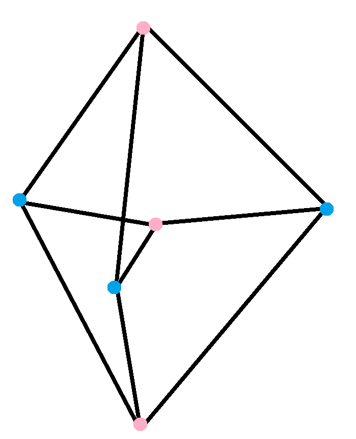
The truncation of the polygon x3-3-o3 requires
that the former 3-edges become "smaller" and that every vertex has locally to be replaced by a "small" copy of its vertex figure,
i.e. a (further) triangle each, connecting to the formerly vertex incident old triangles one by one.
Thus the former vertex count has to be multiplied by 3, while the former edge count becomes doubled.
(Cf.
![]() ).
).
24 | 1 1
---+----
 3 | 8 *
 3 | * 8
or
24 |  2
---+---
 3 | 16
Obviously those "old" and "new" triangles provide a further "outer" symmetry of interchange, hence the group order gets doubled up as well. – As a mere configuration it can also be represented by the Cayley diagram of the binary tetrahedral group, depicted at the right.
It shall be pointed out, that this combinational diagram indeed can be embedded into ico (in a somewhat subsymmetrical way) as follows: consider the latter to be the lace tower oct || co || oct and orient the layer realms (commonly) further in their triangle-first orientations. Then one maps the 2 central blue triangles of the diagram onto the bases of the top antiprism (oct), the 2 central red triangles of the diagram onto the bases of the bottom antiprism (oct). Next consider the central co (within that mentioned orientation) as a further lace tower x3o || x3x || o3x in turn, having a closed edge path of 12 lacing edges, zig-zagging between the upper polar circle (trig) via the equator (hig) to the lower polar circle (opposite dual trig), then up again, etc. This sequence represents the outer dodecagon of the diagram. Color the upper downgoing edges in red, the lower downgoing edges in blue, the lower upgoing edges in red again, and the upper upgoing edges in blue. Now choose that triangle each, incident to either of these upper red edges, which connects by its tip to the upper base of the top oct, connect similarily the lower blue edges each to the respective vertex of the lower base of the bottom oct, then the lower red edges each to the respective vertex of the lower base of the top oct, and finally the upper blue edges each to the respective vertex of the upper base of the bottom oct. The thus constructed 12 triangles will take over the colors of their respective co edges and are the 12 outer triangles of the right diagram. In fact, this embedding selects the top and bottom oct and furthermore those 6 octs form ico, which have a single vertex within the upper and lower layer each, while their equatorial diametral square happens to be a square face of that equatorial co: each of those 8 octs indeed has a pair of diametral triangular faces which got colored thereby. However the 2 colored faces of the top one are both blue, the 2 colored faces of the bottom one are both red, and the 2 colored faces of those connecting ones are one blue, one red each. (All the other 16 octs of ico will have a single face being colored only.)
This real space embedding into ico makes its circumradius evidently 1.
The truncation of the polygons xp-4-o3 and op-4-x3, wrt. the respectively other direction each, then becomes possible as well: In the first case the vertex figure is a 3-edge, thus the formerly g/3 vertices each get streched out into 3, while in the latter case the vertex figure is a p-edge, thus the formerly g/p vertices each get streched out into p, resulting within either case in exactly g vertices. The (complex) edges will be the ones of either of both pre-images.
| x2-4-x3 | x3-4-x3 | x4-4-x3 | x5-4-x3 |
18 | 1 1 ---+---- 2 | 9 * 3 | * 6 |
72 |  1  1
---+------
 3 | 24  *
 3 |  * 24
or 72 | 2 ---+--- 3 | 48 |
288 | 1 1 ----+------ 4 | 72 * 3 | * 96 |
1800 | 1 1 -----+-------- 5 | 360 * 3 | * 600 |
Obviously most of these complex polygons would not be regular, rather being just isogonal. Only within the single case p=3 we have an additional outer symmetry of p=r.
This general class of complex polygons not only fully encompasses xp-4-o2 (herein being the infinite set of cases q=2), but moreover provides a general equivalence on complex polygonal Dynkin diagrams, in fact their incidence matrices happen to read
v |   1   1
--+--------
p | v/p   *
p |   * v/p
or
v |    2
--+-----
p | 2v/p
where v=8p2q/(2p+2q-pq)2. In fact, in the former case of regular diagram representation the given value of v indeed happens to be g1/2, whereas in the second case of non-regular diagram representation one calculates g2=v instead. But that seeming difference indeed is correct, because in the latter case the value of g2 describes the order of the color subgroup with index 2 (left vs. right ringed node) of that group with order g1 (single ringed node only).
Note, that this second representation class also encompasses the general type C for q=2, which in turn was already given explicitely in xp-4-o2 = xp xp, and which thus further evaluates its vertex count into v=p2.
Beyond the afore mentioned infinite subclass, the following 5 cases (of type F in the above list) would belong here particularly (incl. the already individually given case x3-3-x3):
| x3-6-o2 = x3-3-x3 | x4-6-o2 = x4-3-x4 | x5-6-o2 = x5-3-x5 | x3-8-o2 = x3-4-x3 | x3-10-o2 = x3-5-x3 |
24 | 1 1
---+----
 3 | 8 *
 3 | * 8
or 24 | 2 ---+--- 3 | 16 |
96 |  1  1
---+------
 4 | 24  *
 4 |  * 24
or 96 | 2 ---+--- 4 | 48 |
600 |   1   1
----+--------
  5 | 120   *
  5 |   * 120
or 600 | 2 ----+---- 5 | 240 |
72 |  1  1
---+------
 3 | 24  *
 3 |  * 24
or 72 | 2 ---+--- 3 | 48 |
360 |   1   1
----+--------
  3 | 120   *
  3 |   * 120
or 360 | 2 ----+---- 3 | 240 |
Finally some random remarks on real space embeddings. x3-3-x3 already was mentioned (there) to be embeddable into ico. – For x4-3-o4 (there) was mentioned that it is embeddable into gico, i.e. the 5 tes compound with ico as its hull. In fact those x4 edges there are represented by (some) real space squares, then lying diametral within its octs. Its in here asked for truncation thus inserts further x4 edges, i.e. further such real space squares. Those come in by the Stott addition of the dual ico to the former, then resulting in spic, which indeed has exactly 2 such octs per vertex. However, it not is represented by those octs themselves, rather by (some of) their diametral squares. – For x5-3-o5 (there) was mentioned that its vertex set is embeddable into gohi, again representing the x5 edges there by (some) real space pentagons. Its in here asked for truncation thus inserts further x5 edges, i.e. further such real space pentagons. Those come in by the Stott addition of the dual gohi to the former, then resulting in the Grünbaumian polychoron 2sophi or its uniform counterpart sophi. – x3-4-o3 there was mentioned to be embeddable into ico as well. The truncation then here adds the dual ico again, so that we then come to their Stott addition once more, i.e. to spic. In contrast to the other case above in here we use 3-edges each, thence those become represented by (some of) the triangles of their octs. – Right the same interplay should happen within the last case too: The hull of that there obtained sophi is rox, thus the here being used 3-edges ought be represented by (some of) its triangles.
This class obviously represents the dual of the former (when p → r and v → e). Accordingly we get for incidence matrix
2e/r | r
-----+--
   2 | e
where e=8qr2/(2q+2r-qr)2. Again those encompass the infinite subclass x2-4-or as well as the 5 extra cases (of type F in the above list)
| x2-6-o3 | x2-6-o4 | x2-6-o5 | x2-8-o3 | x2-10-o3 |
16 | 3 ---+--- 2 | 24 |
48 | 4 ---+--- 2 | 96 |
240 | 5 ----+---- 2 | 600 |
48 | 3 ---+--- 2 | 72 |
240 | 3 ----+---- 2 | 360 |
Given the real space embedding of their (complex) duals into according polychora and that such a dualization of (complex) polygons is nothing but their rectification, i.e. uses vertices at the centers of the pre-image's edges, within the speech of this embedding it thence uses the new vertices at the centers of the former selected polygons (at least for p>2 there). Sure, the centers of all the 2-dimensional faces of a regular real space polychoron would generally be given by the vertex set of the according bi-rectified polychoron. However, in here the complex edges all happen to be real ones again, so we are left with the (mono-) rectified polychoron instead.
Or, given it differently in turn, the indeed real edges (2-edges) of x2-2q-or simply run between the vertices of xr-q-or and its r-edge centers (then placed somewhat further out to get the same circumradius). This is because the latter complex polytope is selfdual, the vertex figures of both those mentioned polytopes are the same, and the truncation of the latter polytope (i.e. xr-q-xr) is the dual of the former polytope (i.e. of x2-2q-or). If one further notes, that the count of such vertex to edge-center connections in any (complex or real) polygon is just the count of its flags, it becomes clear that the edge count of x2-2q-or just happens to be the group order of xr-q-or.
dual( x2-2q-or ) ≡ rect( x2-2q-or ) = o2-2q-xr = xr-q-xr
Those simply are the truncates (in the respectively other direction) of the former two general classes. Thus the vertex count of xp-2q-o2 just gets doubled up, because every vertex gets replaced by a further normal (real = 2-fold) edge. Conversely the vertex count of x2-2q-or (with r → p) would have to be multiplied by p, because every vertex will get replaced by a further p-edge. At every (new) vertex simply either of those edge types connect one-by-one. And both of either edge types will get taken over.
v |   1   1
--+--------
p | v/p   *
2 |   * v/2
where now v=16p2q/(2p+2q-pq)2. – For the examplified 5 cases (of type F in the above list) one gets especially:
| x3-6-x2 | x4-6-x2 | x5-6-x2 | x3-8-x2 | x3-10-x2 |
48 | 1 1 ---+------ 3 | 16 * 2 | * 24 |
192 | 1 1 ----+------ 4 | 48 * 2 | * 96 |
1200 | 1 1 -----+-------- 5 | 240 * 2 | * 600 |
144 | 1 1 ----+------ 3 | 48 * 2 | * 72 |
720 | 1 1 ----+-------- 3 | 240 * 2 | * 360 |
Again, the remaining infinite sub-class (for q=2) already has been given separately by xp-4-x2.
Obviously all these complex polygons would not be regular, rather they are just isogonal.
The snub of a real polygon is obtained by replacing any alternate vertex, i.e. every pair of subsequent sides incident to it, by a single edge underneath. Within x2-2q-or we have an even count of vertices, which thus can be "alternated", we also still have real edges, but this time r per vertex. Thence the sectioning facet underneath will have to be a (complex) r-edge instead. On the other hand we still consider polygons, that is the vertex figure of the remaining vertices remains nothing but the former vertex figure, i.e. those are r-edges too. Therefore the off-diagonal elements of the incidence matrix both have to be r, while the vertex count gets halved. This after all establishes the mentioned equality of symbols, the latter of which already have been provided above in various individual cases for q>2, cf. x3-3-o3, x3-4-o3, x3-5-o3, x4-3-o4, and x5-3-o5 respectively.
(Note however, that q=2 would leave an unringed node in conjunction with a 2-marked link in the latter symbol, which already for real polytopes becomes degenerate and hence should be excluded generally. In fact, the according snub will be considered separately below.)
The starting figure for this snub would be x2-4-or, the real space embedding of which was mentioned to be the r-gon duotegum. Thus both, either by halving the vertex count, or by investigating the vertex figure underneath a to be deleted vertex, which then will be used as a facet (edge) in here, it becomes evident that this snub indeed becomes dimensionally degenerate (as already was proposed above, thence excluding this case from the former): its real space embedding then consists of a single of the 2 spanning r-gons of that duotegum, which, when considered as its complex space meaning, simply results in a single r-edge only. i.e. right that vertex figure of its pre-image.
Note, that this outcome is not different from the real case: s4o (i.e. using r=2 in here) likewise was just a single diametral facet (edge) of its pre-image square x4o. And, just like there, where this new real edge becomes obtained underneath either of the 2 omitted vertices of the pre-image, i.e. where this edge in a first run occurs as a double cover (before it might become considered to get identified), in here too that complex r-edge occurs as a corresponding r-cover: once underneath each omitted vertex of the pre-image.
The starting figure for this snub would be xp-4-o2. The edges of that snub then clearly are the pre-image's vertex figures, which here are the sectioning facets underneath the omitted elements. Accordingly those will be 2-fold edges, i.e. just real ones.
The coordinates of the pre-image there had been given as (εpn, εpm)/(2 sin(π/p)) for any 1≤n,m≤p, where εp=exp(2πi/p). However, so far we had considered snubs only, where the index p of the sp-node had been 2 only, and for all the real space polytopes this likewise had been the case. Here now, for the first time, the pre-image node consists of a p-edge. None the less an according alternation is still possible, but then it is no longer one out of two, rather it is selecting (locally!) one out of p instead.
In fact, this afore mentioned quest amounts in a further relation on those possible exponents of the coordinates: n+m ≡ 0 mod(p). For higher-dimensional generalized Shephard hypercubes as pre-images this modulo process indeed provides complex full-dimensional results. Within this complex 2-dimensional case however, it becomes degenerate. In fact, that complex polygon of the pre-image had there been mentioned to be the vertices and p-gons of the p-gonal duoprism together with their according incidences. Now consider instead, as a representation of the latter, simply the torus of its squares instead, and then cut that one open into a grid of p times p squares (assuming here p>2 for sure). If now one would choose just one out of p vertices each per rows and columns, and moreover shall do it within the mentioned modulo sense, then here this indeed amounts within a single real space (non-skew!) p-gon only: one out of several Clifford parallels, which in turn would represent all the other modulo values.
Therefore the whole snub in this case has circumradius 1/(2 sin(π/p)) and the incidence matrix
p | 2
--+--
2 | p
The case p=2 was already mentioned to be degenerate.
More generally, the vertex count of the pre-image xp-4-o3 shall by divided by p in here. And the edges to be used in here are given by the sectioning facets underneath the former vertices, within other words their vertex figures, which clearly are 3-edges throughout.
From the pictures provided for x3-4-o3 and x3-3-o3 respectively, the latter to be superimposed to the former in a vertex coincident way (i.e. slightly rotated by π/12), it becomes evident that the latter not only re-uses indeed 1/3 of the former's vertices, but all its complex edges are indeed 3-edges. Thence we deduce that s3-4-o3 turns out to be nothing but the latter.
From the right subgroup diagram the above result (for p=3) in conjunction with the already given general remarks finally can be generalized (for p=3,4,5) into: sp-4-o3 results in nothing but x3-p-o3. Not only the according subgroup relation is valid, but also the respective vertex counts as well as the respective edge types match. (The incidence matrices for those have been given already at x3-3-o3, x3-4-o3, and x3-5-o3 respectively.)
Esp. one obtaines thereby the following interesting snub iteration:
snub( snub( x4-4-o3 ) ) ≡ snub( s4-4-o3 ) = snub( x3-4-o3 ) ≡ s3-4-o3 = x3-3-o3
Similarily as above we conclude that the vertex count here always is nothing but 1/3 of that of its pre-image x3-4-or and the new edges generally are the vertex figures of these pre-images, i.e. they are of type r. Putting this together with the above displayed subgroup diagram, we deduce that s3-4-or results in nothing but xr-3-or. (The incidence matrices for those have been given already at x2-3-o2, x3-3-o3, x4-3-o4, and x5-3-o5 respectively.)
Despite being not even an isogonal complex polygon, because the vertices of its 2 bases clearly do not interchange, the fact that its lacing edges are still real ones makes it to an easily understood polygon. In fact, its real space embedding happens to become real 3-dimensional only and is nothing but a p-gonal pyramid: re-using its real base face in here as a p-edge, keeping the lacing edges additionally, as well as all its vertices. (Within the extremal case of p=2 this complex polygon degenerates into the real triangle, then however gaining further symmetries and thereby becoming regular again.)
Hence its incidence matrix simply becomes
1 * | p 0
* p | 1 1
----+----
1 1 | p *
0 p | * 1
From its real space embedding its circumradius is obtained as 1/sqrt[4-1/sin2(π/p)].
For those lace prisms their 2 bases however do interchange by means of a top-down symmetry. Accordingly this complex polygon at least becomes isogonal. The lacing edges are still real ones. Again its real space embedding happens to become real 3-dimensional only and is nothing but the uniform p-gonal prism: re-using their real base faces in here as a p-edges, keeping the lacing edges additionally, as well as all its vertices. (Within the extremal case of p=2 this complex polygon degenerates into the real square, i.e. gaining further symmetries and thereby becoming regular again.)
Hence the incidence matrix simply becomes
p * | 1 1 0
* p | 0 1 1
----+------
p 0 | 1 * *
1 1 | * p *
0 p | * * 1
or
2p | 1 1
---+----
 p | 2 *
 2 | * p
From its real space embedding its circumradius is obtained as sqrt[1/4-1/(4 sin2(π/p))].
After all, H.S.M. Coxeter notes, that, in order to exist as a complex polygon xp-q-or, there has to be an according Schwarz triangle of the form (p, 2q, r), subject to p,r being integral. This observation then esp. would allow for regular complex star polygons as well. – This is based on E. Hess' theorem, which states that regular starry polytopes always have coinciding vertex sets with according non-starry ones. It further is due to P. McMullen that this theorem can be proven generally, i.e. without considering each individual case. And as such it then applies to complex polytopes as well.
Note, that for those then the previous restriction (i.e. if q is odd, then p=r) no longer applies. (In fact, in order to emphasize this very fact P. McMullen likes to rewrite such q=n/d with n odd rather by q=m/b, with m=2n and b=2d instead. Because then that m would become even again. Furthermore it would be this m, which applies to the according generator equation (AB)m/2 = (BA)m/2.)
| starry | |||||
|---|---|---|---|---|---|
|
o3-3-o2 or: o3-6/2-o2 |
o4-3-o2 or: o4-6/2-o2 |
o5-3-o2 or: o5-6/2-o2 |
o5-3-o3 or: o5-6/2-o3 |
o3-5-o2 or: o3-10/2-o2 |
o5-5-o2 or: o5-10/2-o2 |
x3-3-o2 o3-3-x2 x3-3-x2 *) |
x4-3-o2 o4-3-x2 x4-3-x2 *) |
x5-3-o2 o5-3-x2 x5-3-x2 *) |
x5-3-o3 o5-3-x3 x5-3-x3 *) |
x3-5-o2 o3-5-x2 x3-5-x2 *) |
x5-5-o2 o5-5-x2 x5-5-x2 *) |
|
o3-5/2-o2 or: o3-10/4-o2 | o3-5/2-o3 |
o5-5/2-o3 or: o5-10/4-o3 | o5-5/2-o5 | o3-8/3-o2 | o3-8/3-o4 |
x3-5/2-o2 o3-5/2-x2 x3-5/2-x2 *) |
x3-5/2-o3 x3-5/2-x3 |
x5-5/2-o3 o5-5/2-x3 x5-5/2-x3 *) |
x5-5/2-o5 x5-5/2-x5 |
x3-8/3-o2 o3-8/3-x2 x3-8/3-x2 *) |
x3-8/3-o4 o3-8/3-x4 x3-8/3-x4 *) |
| o3-10/3-o2 | o5-10/3-o2 | o5-10/3-o3 | o2-n/d-o2 | ||
x3-10/3-o2 o3-10/3-x2 x3-10/3-x2 *) |
x5-10/3-o2 o5-10/3-x2 x5-10/3-x2 *) |
x5-10/3-o3 o5-10/3-x3 x5-10/3-x3 *) |
x2-n/d-o2 x2-n/d-x2 | ||
*) The ones marked such are not regular complex polygons, they rather are just isogonal ones only. In fact, the outer symmetry between their edges xp and xr would be missing.
However, for the starry ones much less effort is needed, simply because, just as for real space polytopes too, the (symmetry based) incidence matrix does not involve any dependancy of the subfactors of the link marks. For instance the incidence matrix of x3-3-o2 = x3-6/2-o2 is exactly the same as that of x3-6-o2. It is just that their geometric realizations would differ.
According to P. McMullen that q=3 here ought be rewritten as q=6/2, not only to solve the problem about an according odd value while simultaneously having p≠r, but also the girth can be seen in the left picture to be a double wound hexagon (outlined by the black dots).
But then it simply becomes the conjugate to x3-6-o2. And indeed, the right picture shows 24 vertices as well as 12 small (blue) plus 4 large (red) triangles, just as that incidence matrix requires: The triangles (here representing 3-edges) everywhere are incident by 2 each.
24 |  2
---+---
 3 | 16
This complex star polygon surely has the same incidence matrix as was already given for x3-5-o3. However, its real space embedding would be into gax instead.
120 |   3
----+----
  3 | 120
This complex star polygon, alike x3-5-o3, x5-3-o5, and x3-5/2-o3, . would have for its real space embedding an ex faceting too. In fact, in here it happens to be gaghi.
From the thus given vertex count and the given p-adicity of its edges it follows that its incidence matrix coincides after all with that of x5-3-o5.
120 |   5
----+----
  5 | 120
The variety of (true) complex polyhedra is best be organised in the following table with links to individual files each, because such a table shows more clearly the respective Wythoffian relationships within each familly.
| o3-3-o3-3-o3 | o3-3-o3-4-o2 | op-4-o2-3-o2 | some prismatics | some lace prisms †) |
|---|---|---|---|---|
x3-3-o3-3-o3 (Hessian polyhedron) o3-3-x3-3-o3 x3-3-x3-3-o3 x3-3-o3-3-x3 x3-3-x3-3-x3 |
x3-3-o3-4-o2 o3-3-x3-4-o2 o3-3-o3-4-x2 x3-3-x3-4-o2 x3-3-o3-4-x2 *) o3-3-x3-4-x2 *) x3-3-x3-4-x2 *) o3-3-o3-4-s2 |
xp-4-o2-3-o2 (γp3, Shephard's generalised cube) op-4-x2-3-o2 op-4-o2-3-x2 (βp3, Shephard's generalised oct) xp-4-x2-3-o2 *) xp-4-o2-3-x2 *) op-4-x2-3-x2 xp-4-x2-3-x2 *) sp-4-o2-3-o2 ( (γp3)/p ) |
xp x3-3-o3 *) xp x2-3-o2 *) xp xr-4-o2 *) xp xp-4-o2 x2 x2-4-or xp xr xt *) xp xp xp |
xp xr || op xr x3-3-o3 || o3-3-x3 |
*) The ones marked such are not (generally) uniform complex polyhedra, they (then) rather are just isogonal ones only.
In fact, these would include at least some isogonal-only complex polygons for faces.
†) lacing facets usually would not even be isogonal.
Coxeter esp. points out the close analogy between the 3 complex polyhedra o3-3-o3-4-x2, x3-3-o33-o3, and x3-3-o3-4-o2 on the one side and the 3 real space polyhedra o2-3-o2-4-x2 (cube), x2-3-o2-3-o2 (tet), and x2-3-o2-4-o2 (oct) on the other side: in the first each we have as its vertex set 2 mutually inverted copies of those of the second ones, while the vertices of the third each are the centers of the edges of the second. Moreover first and last are obviously vice versa's duals.
Finally Coxeter shows that there will be neither further truely complex regular polyhedra nor any truely complex regular star polyhedra either. And, by "telescoping" the possible facet groups with the possible vertex figure groups, it becomes evident, that thus esp. the latter will be true for any higher dimension as well.
The variety of complex polychora is best be organised in the following table with links to individual files each, because such a table shows more clearly the respective Wythoffian relationships within each familly.
| o3-3-o3-3-o3-3-o3 | op-4-o2-3-o2-3-o2 | some prismatics |
|---|---|---|
x3-3-o3-3-o3-3-o3 (Witting polychoron) o3-3-x3-3-o3-3-o3 x3-3-x3-3-o3-3-o3 x3-3-o3-3-x3-3-o3 x3-3-o3-3-o3-3-x3 o3-3-x3-3-x3-3-o3 x3-3-x3-3-x3-3-o3 x3-3-x3-3-o3-3-x3 x3-3-x3-3-x3-3-x3 |
xp-4-o2-3-o2-3-o2 (γp4, Shephard's generalised tes) op-4-x2-3-o2-3-o2 op-4-o2-3-x2-3-o2 op-4-o2-3-o2-3-x2 (βp4, Shephard's generalised hex) xp-4-x2-3-o2-3-o2 *) xp-4-o2-3-x2-3-o2 *) xp-4-o2-3-o2-3-x2 *) op-4-x2-3-x2-3-o2 op-4-x2-3-o2-3-x2 op-4-o2-3-x2-3-x2 xp-4-x2-3-x2-3-o2 *) xp-4-x2-3-o2-3-x2 *) xp-4-o2-3-x2-3-x2 *) op-4-x2-3-x2-3-x2 xp-4-x2-3-x2-3-x2 *) sp-4-o2-3-o2-3-o2 ( (γp4)/p ) |
xp xp-4-o2-3-o2 xp-4-o2 xp-4-o2 xp xp xp-4-o2 xp xp xp xp |
*) The ones marked such are not uniform complex polychora, they rather are just isogonal ones only. In fact, these would include at least some isogonal-only complex polygons for faces.
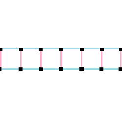
Within real space there was just a single 1-dimensional tiling x2-∞-o2 ≅ x2-∞-x2. However within complex 1-dimensional space there is a lot more freedom. From their relation towards the Schwarz triangles, as was mentioned for the complex polygons, this amounts in here that p,r have to be one of the pairs: 2,2 (which was already mentioned); 3,2; 3,3; 4,2; 4,4; 6,2; 6,3; 6,6; or one of their reversions. Within δp,r2 = xp-q-or , for their according value of q one in here surely has additionally
1/p + 2/q + 1/r = 1
Even an extrapolation according to p → ∞ seems possible in here. However, when considering such cases it becomes evident, that such nodes need to be ringed. In fact, else the seed point itself would be infinitely far away. Thence we get alltogether the following 1-dimensional complex tilings:
|
o2-∞-o2 (real ones) | o4-4-o4 | o6-3-o6 | o∞-2-o∞ |
|---|---|---|---|
x2-∞-o2 x2-∞-x2 |
x4-4-o4 x4-4-x4 |
x6-3-o6 x6-3-x6 |
x∞-2-x∞ |
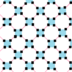
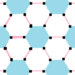
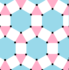
| o3-12-o2 | o4-8-o2 | o6-6-o2 | o∞-4-o2 |
x3-12-o2 o3-12-x2 x3-12-x2 *) |
x4-8-o2 o4-8-x2 x4-8-x2 *) |
x6-6-o2 o6-6-x2 x6-6-x2 *) |
x∞-4-o2 x∞-4-x2 *) |
| o3-6-o3 | o6-4-o3 |
o∞-3-o3 or: o∞-6/2-o3 | |
x3-6-o3 x3-6-x3 |
x6-4-o3 o6-4-x3 x6-4-x3 *) |
x∞-3-o3 x∞-3-x3 *) |
*) The ones marked such are not regular complex tilings, they rather are just isogonal ones only. In fact, the outer symmetry between their edges xp and xr would be missing.
These happen to be the vertices and the real p-gons (then representing complex p-edges) of the real space tilings o-p-x-q-o., i.e.
| x3-12-o2 = x3-6-x3 | x4-8-o2 = x4-4-x4 | x6-6-o2 = x6-3-x6 | x∞-4-o2 = x∞-2-x∞ |
(all vertices and all x3o of that) |
(all vertices and all x4o of sha) |
(all vertices and all x6o of that) |
(all vertices and all x∞o of sha) |
|
| |||
(N → ∞) 3N | 2 ---+--- 3 | 2N |
(N → ∞) 2N | 2 ---+-- 4 | N |
(N → ∞) 3N | 2 ---+-- 6 | N |
(N,M → ∞) NM | 2 ---+--- M | 2N |
(N → ∞) 3N | 1 1 ---+---- 3 | N * 3 | * N |
(N → ∞) 4N | 1 1 ---+---- 4 | N * 4 | * N |
(N → ∞) 6N | 1 1 ---+---- 6 | N * 6 | * N |
(N,M,K → ∞) NMK | 1 1 ----+------ M | NK * K | * NM |
The last row within the above table then derives from the above given second, i.e. truncated symbols. That operation then applies onto the pre-images, where just the first node each would be ringed instead. Those then are x3-6-o3, x4-4-o4, and x6-3-o6 respectively. (As mentioned already above, a non-truncated pre-image for the last column does not exist.) Note that their pictures would be derived from the above given ones by extending every alternate p-gon (complex p-edge) to the neighbouring ones centers each. That is, in converse, the above pics indeed are derived from those pre-images by inserting further p-gons (complex p-edges) in between: right those other alternates, which come in here as the pre-image's vertex figures.
These dual ones of the formers happen to be the vertices and the real edges (then representing complex 2-edges) of the real space tilings x-q-o-r-o., i.e.
| x2-12-o3 | x2-8-o4 | x2-6-o6 |
(all vertices and all edges of hexat) |
(all vertices and all edges of squat) |
(all vertices and all edges of trat) |
|
| ||
(N → ∞) 2N | 3 ---+--- 2 | 3N |
(N → ∞) N | 4 --+--- 2 | 2N |
(N → ∞) N | 6 --+--- 2 | 3N |
The case x∞-4-o2 was already considered above within a different grouping. The remaining ones then happen to be the vertices and the real p-gons (then again representing complex p-edges) of the real space tilings x-p-o-r-o., i.e.
| x3-4-o6 | x4-4-o4 | x6-4-o3 |
(all vertices and all x3o of trat) |
(all vertices and all x4o of squat) |
(all vertices and all x6o of hexat) |
(N → ∞) N | 6 --+--- 3 | 2N |
(N → ∞) N | 4 --+-- 4 | N |
(N → ∞) 2N | 3 ---+-- 6 | N |
This one happens to be obtained by the vertices and the alternate real triangles (then again representing complex 3-edges) of trat.
(N → ∞)

N | 3
--+--
3 | N
(all vertices and
This one looks like being obtained from trat again. But rather it is obtained instead from ghat (old: fexat, the 3-hexat-compound): in fact, at every vertex there are exactly 6 hexagons (i.e. complex 6-edges) and each girth has length 3.
Note furthermore, that, by neglecting the real edges within the complex incidence structure, this dubious property, of being derived from a real space compound, becomes lost. Rather it indeed happens to be a fully valid complex polgon.
(N → ∞)

N | 6
--+--
6 | N
This one looks like being obtained from trat once more. But this time the link mark q=3 is odd while the node marks are different p≠r. According to P. McMullen this can be solved by using the non-reduced form q=6/2 instead. I.e. the girth in here happens to be a Grünbaumian double cover sequance of -red-green-cyan-red-green-cyan- instead. Thus the edges of that "trat" happen to be local double covers, and the vertices even are triple covers of mutually gyrated, X-shaped that vertex configurations instead. Thus in x∞-6/2-o3 the complex ∞-edges therefore happen to be double covers of all the azes of tha. And x∞-3-o3 then would just represent its reduced, non-Grünbaumian form.
(N,M → ∞)

NM |  3
---+---
 M | 3N
Beyond the mere regular ones those truncations derive from the polygons xp-2q-o2 and op-2q-x2, via Stott expansion wrt. the respectively other direction each. In the first case the vertex figure is a 2-edge, thus the previous vertex count gets doubled, while in the second case the vertex figure is a p-edge, thus the previous vertex count there gets multiplied by p (which surely comes out to be the same). The complex edges on the other hand will get be re-used both, alternatingly. Thus their incidence matrices clearly read
| x3-12-x2 | x4-8-x2 | x6-6-x2 | x∞-4-x2 |
|
|
|
|
(N → ∞) 6N | 1 1 ---+------ 3 | 2N * 2 | * 3N |
(N → ∞) 4N | 1 1 ---+----- 4 | N * 2 | * 2N |
(N → ∞) 6N | 1 1 ---+----- 6 | N * 2 | * 3N |
(N,M → ∞) NM | 1 1 ---+----- M | N * 2 | * NM |
The last case of p → ∞ indeed could be derived within this limiting process only: Just consider the cyan shapes (p-edges) getting larger, while the white shapes (holes) getting smaller.
Obviously none of these complex tilings would not be regular, rather they are just isogonal.
Those truncations derive quite similarily as in the former consideration from their respective pre-images. However, in here the medial case was already considered above: x4-4-x4. And the other two pre-images will be each others Stott expansion. Thus this case just results in a single (additional) outcome.
(N → ∞)

6N |  1 1
---+-----
 3 | 2N *
 6 |  * N
Obviously this complex polygon would not be regular, rather it is just isogonal.
This then is the truncation of x∞-3-o3, i.e. its Stott expansion wrt. its second node. As a local configuration it surely consists of a ∞-edge and a 3-edge, incident at a vertex, as being represented within real space by a triangle and a vertex-incident tangent to its circum-sphere (i.e. ace). However, as was outlined within its non-truncated form already, the odd link mark q=3 in context with non-equal node marks p≠r results in an identification of 2 such completely coincident aces for its resolution as q=6/2, i.e. within the reduction this local configuration rather would look like one ace with a tip-incident triangle on either side. However, this still would require 3 mutally gyrated copies at each vertex. In fact, within q=6/2 it is more like six of the former one-sided local configurations for that Grünbaumian pre-image. Thence thats incidence matrix indeed would read like
(N,M → ∞)

6NM |  1   1
----+-------
  M | 6N   *
  3 |  * 2NM
or
3NM |  1  1
----+------
  M | 3N  *
  3 |  * NM
wrt. some redefined N, eating up the former common factor. But obviously, vertices then coincide by 6 and ∞-edges by 2.
Furthermore this complex polygon would not be regular either, rather it is just isogonal.
We might conclude, that, after all, the incidence matrices of the regular complex tilings happen to be independent of q. In fact, any such δp,r2 := xp-q-or has for matrix just
(N → ∞)

pN |  r
---+---
 p | rN
Same independance of q applies for the truncated complex tilings, i.e. any such xp-q-xr has for matrix
(N → ∞)

prN |  1  1
----+------
  p | rN  *
  r |  * pN
(In the individual matrices above it just was that a possible common factor had been subsumed into that N → ∞.) This observed independence of q clearly could be supported from the fact that q = 2pr/(pr-p-r) is not a free variable in here, and thus in any of its possible occurences it further could be decomposed into the other 2 variables instead.
First we have to note, that the comb product of any pair of 1-dimensional tilings δp,r2 = xp-q-or would result in a 2-dimensional tiling comb( δp1,r12, δp2,r22 ) = comb( xp1-q1-or1, xp2-q2-or2 ). As already was mentioned at the end of the former section, that one does not depend on either of their link marks qk then too. For sure, within this general setting, most of such tilings would be isogonal only.
Moreover, an according product of any 1-dimensional regular tiling with itself indeed would result in a then regular 2-dimensional tiling. As it turns out, those will happen to become δp,r3 := comb( δp,r2, δp,r2 ) = comb( xp-q-or, xp-q-or ) = xp-4-o2-4-or.
| op1-q1-or1 op2-q2-or2 | |||||
|---|---|---|---|---|---|
xp1-q1-or1 xp2-q2-or2 (δp1,r12 × δp2,r22) *) xp1-q1-xr1 xp2-q2-or2 *) xp1-q1-xr1 xp2-q2-xr2 *) cases: pk,qk,rk (k = 1,2) = (2,∞,2;) 2,12,3; 2,8,4; 2,6,6; 3,12,2; 3,6,3; -- 3,4,6; 4,8,2; -- 4,4,4; -- 6,6,2; 6,4,3; -- 6,3,6 | |||||
| op-4-o2-4-or | o2-4-op-4-o2 | o3-3-o3-4-o3 | o4-3-o4-3-o4 | o4-3-o4-4-o2 | |
xp-4-o2-4-or (δp,r3) op-4-x2-4-or xp-4-x2-4-or *) xp-4-o2-4-xr *) xp-4-x2-4-xr *) cases: p,r = (2,2;) 2,3; 2,4; 2,6; 3,2; 3,3; -- 3,6; 4,2; -- 4,4; -- 6,2; 6,3; -- 6,6 |
esp.: xp-4-o2-4-op (δp,p3) op-4-x2-4-op xp-4-x2-4-op *) xp-4-o2-4-xp xp-4-x2-4-xp *) xp-4-o2-4-o2 (δp,23) op-4-x2-4-o2 op-4-o2-4-x2 xp-4-x2-4-o2 *) xp-4-o2-4-x2 *) op-4-x2-4-x2 xp-4-x2-4-x2 *) |
x2-4-op-4-o2 o2-4-xp-4-o2 x2-4-xp-4-o2 *) x2-4-op-4-x2 x2-4-xp-4-x2 *) cases: p = (2,) 3, 4, 6 |
x3-3-o3-4-o3 o3-3-x3-4-o3 o3-3-o3-4-x3 x3-3-x3-4-o3 x3-3-o3-4-x3 o3-3-x3-4-x3 x3-3-x3-4-x3 |
x4-3-o4-3-o4 o4-3-x4-3-o4 x4-3-x4-3-o4 x4-3-o4-3-x4 x4-3-x4-3-x4 |
x4-3-o4-4-o2 o4-3-x4-4-o2 o4-3-o4-4-x2 x4-3-x4-4-o2 x4-3-o4-4-x2 *) o4-3-x4-4-x2 *) x4-3-x4-4-x2 *) |
*) The ones marked such are not (or not generally) uniform complex honeycombs, they (then) rather are just isogonal ones only. In fact, these would include at least some isogonal-only complex polygons for faces.
Interestingly it happens that for the truely complex 2-dimensional tilings δp,p3 there are sequences of 4 consecutive rectifications possible, in fact all the same for any p=3,4,6. (The first 2 steps there still keep regularity, the third step keeps at least isogonality as well as isotoxality, while the fourth then keeps isogonality only.)
xp-4-o2-4-op ↓ rectify op-4-x2-4-op ↓ rectify xp-4-o2-4-xp |
= = |
x2-4-op-4-o2 ↓ rectify o2-4-xp-4-o2 ↓ rectify x2-4-op-4-x2 |
= = |
xp-4-o2-4-o2 ↓ rectify op-4-x2-4-o2 ↓ rectify xp-4-o2-4-x2 |
© 2004-2026 | top of page |